Download
1 / 45
450 likes | 601 Views
IDL 102 (Particle Tracking). Our MO. Convert Image DV -> gdf Do not byte-scale Also, do byte scale (after conversion) Find dots in each frame “Clean” image Find all candidate dots Refine dots set Link dots frame-to-frame to get trajectories How far are we willing to look for a particle?

E N D
Our MO • Convert Image DV -> gdf • Do not byte-scale • Also, do byte scale (after conversion) • Find dots in each frame • “Clean” image • Find all candidate dots • Refine dots set • Link dots frame-to-frame to get trajectories • How far are we willing to look for a particle? • How about gaps? • How about blinky, random noise?
Conversion isn’t futile • Images are acquired at 16bit (0 -> 216=65536) • Images have to be displayed at 8bit (0 -> 28=256)
Conversion isn’t futile • Images are acquired at 16bit (0 -> 216=65536) • Images have to be displayed at 8bit (0 -> 28=256)
Conversion isn’t futile • Images are acquired at 16bit (0 -> 216=65536) • Images have to be displayed at 8bit (0 -> 28=256)
Pre-tracking • Find dots in each frame • “Clean” image • Find all candidate dots • Refine dots set
You need to refine them using reasonable criteria X Y Mass Radius Eccentricity Time 0 1 2 3 4 5 0 3 4 5 6 7 0 1 8 9 10 11 12 0 2 13 14 15 16 17 0 3 18 19 20 21 22 0 4 23 24 25 26 27 2 5 28 29 30 31 32 2 6 33 34 35 36 37 3 7 38 39 40 41 42 4 8 43 44 45 46 47 5 9 48 49 50 51 52 5 10 53 54 55 56 57 5 11 58 59 60 61 62 5 12 63 64 65 66 67 6 13 68 69 70 71 72 12 14 73 74 75 76 77 12
Criteria • X, Y can be used to clip edges, where things usually go wrong • “Mass” is total integrated brightness in each blob • Radius of gyration is a measure of size that makes dimmer pixels count less • Eccentricity: • 0: a perfect disk • 1: a perfect line segment • Use eclip.pro, where(), or edgeclip.pro to refine ranges of these criteria
A few things you can use to evaluate your pretracking: • Say your pretracked data is in ‘pt’ • Overview: • ptexplore, pt • Number of particles at each frame (bleaching?) • plot_hist, pt[5,*], bin=1 • Bias towards integer pixel positions • plot_hist, pt[0:1,*] mod 1, bin=.05
Now track them! • User defined params for tracking: • Distance to look for same particle frame-to-frame • This must me less than interparticle distance in each frame • Number of frames a particle is allowed to disappear • This must be less than time it takes for two particles to switch position • Shortest trajectory you consider real • This is a toughie. But setting this to something >0 helps get rid of artifacts that blink
Check tracking with • P(dx, dt=1)
Check tracking with • P(dx, dt=1)
Check tracking with • P(dx, dt=1)
AnalyzeMean squared displacement (MSD) 7 4 9 11 2 t=1 13 10 6 12 5 15 14 3 8
AnalyzeMean squared displacement (MSD) 7 4 9 11 2 t=1 13 10 6 12 5 15 14 3 8 • Measure all displacements that are Dt = 1 frame apart • Square them • Average them • Average over other particles if desired and “allowed” MSD(mm2) 1 13 Dt (frames)
AnalyzeMean squared displacement (MSD) 7 4 9 11 2 t=1 13 10 6 12 5 15 14 3 8 • Measure all displacements that are Dt = 1 frame apart • Square them • Average them • Average over other particles if desired and “allowed” MSD(mm2) • Then do it for Dt = 2 framesand so on 1 2 13 Dt (frames)
Says Einstein! constant in biology y = m x x m= D1 m= D2 MSD(mm2) Dt (frames)
A Yes/No test for diffusion(What’s this about logs and slopes of 1?)
A Yes/No test for diffusion(What’s this about logs and slopes of 1?) 1 1 y = c + m x x 2
Ballistic motion(that of projectiles) Constant velocity gives a slope 2 on a log-log plot