Download
1 / 101
1.08k likes | 1.43k Views
4. Applications of the First Derivative Applications of the Second Derivative Curve Sketching Optimization I Optimization II. Applications of the Derivative. 4.1. Applications of the First Derivative. Increasing and Decreasing Functions.

E N D
4 • Applications of the First Derivative • Applications of the Second Derivative • Curve Sketching • Optimization I • Optimization II Applications of the Derivative
4.1 Applications of the First Derivative
Increasing and Decreasing Functions • A function f is increasing on an interval(a, b) if for any two numbers x1 and x2 in (a, b), f(x1) < f(x2) wherever x1<x2. y f(x2) f(x1) x a x1 x2 b
Increasing and Decreasing Functions • A function f is decreasing on an interval(a, b) if for any two numbers x1 and x2 in (a, b), f(x1) > f(x2) wherever x1<x2. y f(x1) f(x2) x a x1 x2 b
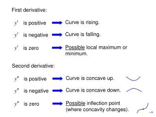
Theorem 1 • If f ′(x) > 0 for each value of x in an interval (a, b), then f is increasing on (a, b). • If f ′(x) < 0 for each value of x in an interval (a, b), then f is decreasing on (a, b). • If f′(x) = 0 for each value of x in an interval (a, b), then f is constant on (a, b).
Example • Find the interval where the function f(x) = x2 is increasing and the interval where it is decreasing. Solution • The derivative of f(x) = x2 is f′(x) = 2x. • f ′(x) = 2x > 0 if x > 0 and f ′(x) = 2x < 0 if x < 0. • Thus, f is increasing on the interval(0, ) and decreasing on the interval(–, 0). y f(x) = x2 Example 1, page 245
Determining the Intervals Where a Function is Increasing or Decreasing • Find all the values ofx for which f ′(x) = 0 or f ′is discontinuous and identify the open intervals determined by these numbers. • Select a test numberc in each interval found in step 1 and determine the sign of f ′(c) in that interval. • If f ′(c) > 0, fis increasing on that interval. • If f ′(c) < 0, fis decreasing on that interval.
Examples • Determine the intervals where the function f(x) = x3 – 3x2 – 24x + 32 is increasing and where it is decreasing. Solution • Find f ′ and solve for f ′(x) = 0: f ′(x) = 3x2 – 6x – 24 = 3(x + 2)(x – 4) = 0 • Thus, the zeros of f ′ are x = –2 and x = 4. • These numbers divide the real line into the intervals(–, –2), (–2, 4), and (4, ). Example 2, page 246
Examples • Determine the intervals where the function f(x) = x3 – 3x2 – 24x + 32 is increasing and where it is decreasing. Solution • To determine the sign of f ′(x) in the intervals we found (–, –2), (–2, 4), and (4, ), we computef ′(c)at a convenient test point in each interval. • Lets consider the values –3, 0,and 5: f ′(–3) = 3(–3)2 – 6(–3) – 24 = 27 +18 – 24 = 21 > 0 f ′(0) = 3(0)2 – 6(0) – 24 = 0 +0 – 24 = –24 < 0 f ′(5) = 3(5)2 – 6(5) – 24 = 75 – 30 – 24 = 21 > 0 • Thus, we conclude that f is increasing on the intervals(–, –2), (4, ), and is decreasing on the interval(–2, 4). Example 2, page 246
Examples • Determine the intervals where the function f(x) = x3 – 3x2 – 24x + 32 is increasing and where it is decreasing. Solution • So, f increases on (–, –2), (4, ), and decreases on (–2, 4): y 60 40 20 –20 –40 –60 y = x3 – 3x2 – 24x + 32 x –7 –5 –3 –1 1 3 5 7 Example 2, page 246
Examples • Determine the intervals where is increasing and where it is decreasing. Solution • Find f ′ and solve for f ′(x) = 0: • f ′(x) = 0 when the numerator is equal to zero, so: • Thus, the zeros of f ′are x = –1 and x = 1. • Also note that f ′ is not defined at x = 0, so we have four intervals to consider: (–, –1), (–1, 0), (0, 1), and (1, ). Example 4, page 247
Examples • Determine the intervals where is increasing and where it is decreasing. Solution • To determine the sign of f ′(x) in the intervals we found (–, –1), (–1, 0), (0, 1), and (1, ), we computef ′(c)at a convenient test point in each interval. • Lets consider the values –2, –1/2, 1/2,and 2: • So f is increasing in the interval (–, –1). Example 4, page 247
Examples • Determine the intervals where is increasing and where it is decreasing. Solution • To determine the sign of f ′(x) in the intervals we found (–, –1), (–1, 0), (0, 1), and (1, ), we computef ′(c)at a convenient test point in each interval. • Lets consider the values –2, –1/2, 1/2,and 2: • So f is decreasing in the interval (–1, 0). Example 4, page 247
Examples • Determine the intervals where is increasing and where it is decreasing. Solution • To determine the sign of f ′(x) in the intervals we found (–, –1), (–1, 0), (0, 1), and (1, ), we computef ′(c)at a convenient test point in each interval. • Lets consider the values –2, –1/2, 1/2,and 2: • So f is decreasing in the interval (0, 1). Example 4, page 247
Examples • Determine the intervals where is increasing and where it is decreasing. Solution • To determine the sign of f ′(x) in the intervals we found (–, –1), (–1, 0), (0, 1), and (1, ), we computef ′(c)at a convenient test point in each interval. • Lets consider the values –2, –1/2, 1/2,and 2: • So f is increasing in the interval (1, ). Example 4, page 247
Examples • Determine the intervals where is increasing and where it is decreasing. Solution • Thus, f isincreasing on (–, –1) and (1, ), anddecreasingon (–1, 0)and(0, 1): y 4 2 –2 –4 x –4 –2 2 4 Example 4, page 247
Relative Extrema • The first derivative may be used to help us locatehigh points and low points on the graph of f: • High points are called relative maxima • Low points are called relative minima. • Both high and low points are called relative extrema. Relative Maxima y y = f(x) Relative Minima x
Relative Extrema Relative Maximum • A function f has a relative maximum at x = c if there exists an open interval (a, b) containing c such that f(x) f(c) for all x in (a, b). Relative Maxima y y = f(x) x x1 x2
Relative Extrema Relative Minimum • A function f has a relative minimum at x = c if there exists an open interval (a, b) containing c such that f(x) f(c) for all x in (a, b). y y = f(x) Relative Minima x x3 x4
Finding Relative Extrema • Suppose that f has a relative maximum at c. • The slope of the tangent line to the graph must change frompositivetonegative as x increases. • Therefore, thetangent line to the graph of fat point(c, f(c))must be horizontal, so that f ′(x)= 0 orf ′(x)is undefined. f ′(x)> 0 y f ′(x)= 0 f ′(x)< 0 x c b a
Finding Relative Extrema • Suppose that f has a relative minimum at c. • The slope of the tangent line to the graph must change fromnegativetopositive as x increases. • Therefore, thetangent line to the graph of fat point(c, f(c))must be horizontal, so that f ′(x)= 0 orf ′(x) is undefined. y f ′(x)> 0 f ′(x)< 0 f ′(x)= 0 x c b a
Finding Relative Extrema • In some cases a derivative does not exist for particular values of x. • Extrema may exist at such points, as the graph below shows: Relative Maximum y Relative Minimum x b a
Critical Numbers • We refer to a number in the domain of f that may give rise to a relative extremum as a critical number. Critical number of f • A critical number of a function f is any number x in the domain of f such that f ′(x)= 0 or f ′(x)does not exist.
Critical Numbers • The graph below shows us several critical numbers. • At points a, b, and c, f ′(x)= 0. • There is a corner at point d, so f ′(x)does not exist there. • The tangent to the curve at point e is vertical, so f ′(x)does not exist there either. • Note that points a, b, and d are relative extrema, while points c and eare not. y Relative Extrema Not Relative Extrema x a b c d e
The First Derivative Test • Procedure for Finding Relative Extrema of a Continuous Function f • Determine the critical numbers of f. • Determine the sign of f ′(x) to the left and right of each critical point. • If f ′(x) changes sign from positive to negative as we move across a critical number c, then f(c) is a relative maximum. • If f ′(x) changes sign from negative to positive as we move across a critical number c, then f(c) is a relative minimum. • If f ′(x)does not change sign as we move across a critical number c, then f(c) is not a relative extremum.
Examples • Find the relative maxima and minima of Solution • The derivative of f is f ′(x) = 2x. • Setting f ′(x) = 0 yields x = 0 as the only critical number of f. • Since f ′(x) < 0 if x < 0 and f ′(x) > 0 if x > 0 we see that f ′(x) changes sign from negative to positive as we move across 0. • Thus, f(0) = 0 is a relative minimum of f. y f(x) = x2 f ′(x) > 0 f ′(x) < 0 Relative Minimum Example 5, page 252
Examples • Find the relative maxima and minima of Solution • The derivative of f is f ′(x) = 2/3x–1/3. • f ′(x) is not defined at x = 0, is continuous everywhere else, and is never equal to zero in its domain. • Thus x = 0 is the only critical number of f. • Since f ′(x) < 0 if x < 0 and f ′(x) > 0 if x > 0 we see that f ′(x) changes sign from negative to positive as we move across 0. • Thus, f(0) = 0 is a relative minimum of f. y 4 2 f(x) = x2/3 f´(x) > 0 f´(x) < 0 x – 4 –2 2 4 Relative Minimum Example 6, page 252
Examples • Find the relative maxima and minima of Solution • The derivative of f and equate to zero: • The zeros of f ′(x) are x = –2 and x = 4. • f ′(x) is defined everywhere, sox = –2 and x = 4 are the onlycritical numbersof f. Example 7, page 253
Examples • Find the relative maxima and minima of Solution • Since f ′(x) > 0 if x < –2 and f ′(x) < 0 if 0 <x < 4, we see that f ′(x) changes sign from positive to negative as we move across –2. • Thus, f(–2) = 60 is a relative maximum. Relative Maximum y 60 40 20 –20 –40 –60 f(x) x –7 –5 –3 –1 1 3 5 7 Example 7, page 253
Examples • Find the relative maxima and minima of Solution • Since f ′(x) < 0 if 0 <x < 4 and f ′(x) > 0 if, x > 4 we see that f ′(x) changes sign from negative to positive as we move across 4. • Thus, f(4) = –48 is a relative minimum. Relative Maximum y 60 40 20 –20 –40 –60 f(x) x –7 –5 –3 –1 1 3 5 7 Relative Minimum Example 7, page 253
4.2 Applications of the Second Derivative
Concavity • A curve is said to be concave upwards when the slope of tangent line to the curve is increasing: • Thus, if f is differentiable on an interval (a, b), then f is concave upwards on (a, b) if f ′is increasing on (a, b). y x
Concavity • A curve is said to be concave downwards when the slope of tangent line to the curve is decreasing: • Thus, if f is differentiable on an interval (a, b), then f is concave downwards on (a, b) if f′is decreasing on (a, b). y x
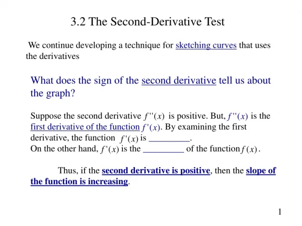
Theorem 2 • Recall that f ″(x) measures the rate of change of the slopef ′(x) of the tangent line to the graph of f at the point (x, f(x)). • Thus, we can use f ″(x) to determine the concavity of f. • If f ″(x) > 0 for each value of x in (a, b), then f is concave upward on (a, b). • If f ″(x) < 0 for each value of x in (a, b), then f is concave downward on (a, b).
Steps in Determining the Concavity of f • Determine the values of x for which f ″is zero or where f ″ is not defined, and identify the open intervals determined by these numbers. • Determine the sign of f ″ in each interval found in step 1. To do this compute f ″(c), where c is any conveniently chosen test number in the interval. • If f ″(c) > 0, fis concave upward on that interval. • If f ″(c) < 0, fis concave downward on that interval.
Examples • Determine where the function is concave upward and where it is concave downward. Solution • Here, and • Setting f ″(c) = 0 we find which gives x = 1. • So we consider the intervals (–, 1) and (1, ): • f ″(x) < 0 when x < 1, so f is concave downward on (–, 1). • f ″(x) > 0 when x > 1, so f is concave upward on (1, ). Example 1, page 265
Examples • Determine where the function is concave upward and where it is concave downward. Solution • The graph confirms that f is concave downward on (–, 1) andconcave upward on (1, ): y 60 40 20 –20 –40 –60 f(x) x –7 –5 –3 –1 1 3 5 7 Example 1, page 265
Examples • Determine the intervals where the function is concave upward and concave downward. Solution • Here, and • So, f ″cannot be zero and is not defined at x = 0. • So we consider the intervals (–, 0) and (0, ): • f ″(x) < 0 when x < 0, so f is concave downward on (–, 0). • f ″(x) > 0 when x > 0, so f is concave upward on (0, ). Example 2, page 266
Examples • Determine the intervals where the function is concave upward and concave downward. Solution • The graph confirms that f is concave downward on (–, 0) andconcave upward on (0, ): Example 2, page 266
Inflection Point • A point on the graph of a continuous function where the tangent line exists and where the concavity changes is called an inflection point. • Examples: y Inflection Point x
Inflection Point • A point on the graph of a continuous function where the tangent line exists and where the concavity changes is called an inflection point. • Examples: y Inflection Point x
Inflection Point • A point on the graph of a continuous function where the tangent line exists and where the concavity changes is called an inflection point. • Examples: y Inflection Point x
Finding Inflection Points To find inflection points: • Compute f ″(x). • Determine the numbers in the domain of f for which f ″(x) = 0 or f ″(x) does not exist. • Determine the sign of f ″(x) to the left and right of each number c found in step 2. If there is a change in the sign of f ″(x) as we move across x= c, then (c, f(c)) is an inflection point of f.
Examples • Find the points of inflection of the function Solution • We have and • So, f ″ is continuous everywhere and is zero for x = 0. • We see that f ″(x) < 0 whenx < 0, and f ″(x) > 0 whenx > 0. • Thus, we find that the graph of f: • Has one and only inflection point at f(0) = 0. • Isconcave downward on the interval (–, 0). • Isconcave upward on the interval (0, ). y f(x) 4 2 –2 –4 Inflection Point x –2 2 Example 3, page 268
Examples • Find the points of inflection of the function Solution • We have and • So, f ″ is not defined at x = 1, and f ″ isnever equal to zero. • We see that f ″(x) < 0 whenx < 1, and f ″(x) > 0 whenx > 1. • Thus, we find that the graph of f: y • Has one and only inflection point at f(1) = 0. • Isconcave downward on the interval (–, 1). • Isconcave upward on the interval (1, ). 3 2 1 –1 –2 –3 f(x) Inflection Point x –2 –1 1 2 Example 4, page 268
Applied Example: Effect of Advertising on Sales • The total salesS(in thousands of dollars) of Arctic Air Co., which makes automobile air conditioners, is related to the amount of money x(in thousands of dollars) the company spends on advertising its product by the formula • Find the inflection point of the function S. • Discuss the meaning of this point. Applied Example 7, page 270
Applied Example: Effect of Advertising on Sales Solution • The first two derivatives of S are given by • Setting S″(x) = 0 gives x = 50. • So (50, S(50)) is the only candidate for an inflection point. • Since S″(x) > 0 for x < 50, and S″(x) < 0 for x > 50, the point (50, 2700) is, in fact, an inflection point of S. • This means that the firm experiences diminishing returns on advertising beyond $50,000: • Every additional dollar spent on advertising increases sales by less than previously spent dollars. Applied Example 7, page 270
The Second Derivative Test • Maxima occur when a curve is concave downwards, while minima occur when a curve is concave upwards. • This is the basis of the second derivativetest: • Compute f ′(x) and f ″(x). • Find all the critical numbers of f at which f ′(x)= 0. • Compute f ″(c), if it exists, for each critical number c. • If f ″(c)< 0, then f has a relative maximum at c. • If f ″(c)> 0, then f has a relative minimum at c. • If f ″(c)= 0, then the test fails (it is inconclusive).
Example • Determine the relative extrema of the function Solution • We have so f ′(x) = 0 gives the critical numbersx = –2 and x = 4. • Next, we have which we use to test the critical numbers: so, f(–2) = 60 is a relative maximum of f. so, f(4) = –48 is a relative minimum of f. Example 9, page 272
4.3 Curve Sketching