Download
1 / 27
270 likes | 295 Views
Dive into optical flow applications, constraints, equations, and solving methods. Learn about the Aperture problem, Lucas-Kanade flow, and robust optical flow techniques. Discover insights, errors, and iterative refinements in flow estimation.

E N D
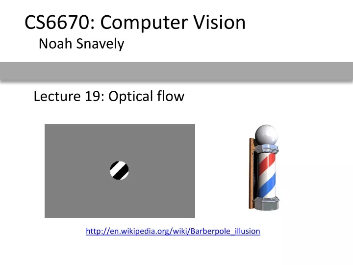
CS6670: Computer Vision Noah Snavely Lecture 19: Optical flow http://en.wikipedia.org/wiki/Barberpole_illusion
Readings • Szeliski, Chapter 8.4 - 8.5
Announcements • Project 2b due Tuesday, Nov 2 • Please sign up to check out a phone! • Final projects • Form a group, write a proposal by next Friday, Oct 29
Optical flow • Why would we want to do this?
Key assumptions • color constancy: a point in H looks the same in I • For grayscale images, this is brightness constancy • small motion: points do not move very far • This is called the optical flow problem Problem definition: optical flow • How to estimate pixel motion from image H to image I? • A more general pixel correspondence problem than stereo • given a pixel in H, look for nearby pixels of the same color in I
Optical flow constraints (grayscale images) • Let’s look at these constraints more closely • brightness constancy: Q: what’s the equation? • small motion: (u and v are less than 1 pixel) • suppose we take the Taylor series expansion of I:
Optical flow equation • Combining these two equations
Optical flow equation • Combining these two equations • In the limit as u and v go to zero, this becomes exact
Optical flow equation • Q: how many unknowns and equations per pixel? • Intuitively, what does this constraint mean? • The component of the flow in the gradient direction is determined • The component of the flow parallel to an edge is unknown This explains the Barber Pole illusion http://www.sandlotscience.com/Ambiguous/Barberpole_Illusion.htm
Solving the aperture problem • Basic idea: assume motion field is smooth • Horn & Schunk [1981]: add smoothness term • Lucas & Kanade [1981]: assume locally constant motion • pretend the pixel’s neighbors have the same (u,v) • Many other methods exist. Here’s an overview: • S. Baker, M. Black, J. P. Lewis, S. Roth, D. Scharstein, and R. Szeliski. A database and evaluation methodology for optical flow. In Proc. ICCV, 2007 • http://vision.middlebury.edu/flow/
Lucas-Kanade flow • How to get more equations for a pixel? • Basic idea: impose additional constraints • Lucas-Kanade: pretend the pixel’s neighbors have the same (u,v) • If we use a 5x5 window, that gives us 25 equations per pixel!
Solution: solve least squares problem • minimum least squares solution given by solution (in d) of: • The summations are over all pixels in the K x K window Lucas-Kanade flow • Prob: we have more equations than unknowns
Conditions for solvability • Optimal (u, v) satisfies Lucas-Kanade equation • When is this solvable? • ATA should be invertible • ATA should not be too small due to noise • eigenvalues l1 and l2 of ATA should not be too small • ATA should be well-conditioned • l1/ l2 should not be too large (l1 = larger eigenvalue)
Observation • This is a two image problem BUT • Can measure sensitivity by just looking at one of the images! • This tells us which pixels are easy to track, which are hard • very useful for feature tracking...
Errors in Lucas-Kanade • What are the potential causes of errors in this procedure? • Suppose ATA is easily invertible • Suppose there is not much noise in the image • When our assumptions are violated • Brightness constancy is not satisfied • The motion is not small • A point does not move like its neighbors • window size is too large • what is the ideal window size?
Iterative Refinement • Iterative Lucas-Kanade Algorithm • Estimate velocity at each pixel by solving Lucas-Kanade equations • Warp H towards I using the estimated flow field • - use image warping techniques • Repeat until convergence
Revisiting the small motion assumption • Is this motion small enough? • Probably not—it’s much larger than one pixel (2nd order terms dominate) • How might we solve this problem?
u=1.25 pixels u=2.5 pixels u=5 pixels u=10 pixels image H image I image H image I Gaussian pyramid of image H Gaussian pyramid of image I Coarse-to-fine optical flow estimation
warp & upsample run iterative L-K . . . image J image I image H image I Gaussian pyramid of image H Gaussian pyramid of image I Coarse-to-fine optical flow estimation run iterative L-K
Robust methods • L-K minimizes a sum-of-squares error metric • least squares techniques overly sensitive to outliers Error metrics quadratic truncated quadratic lorentzian
first image quadratic flow lorentzian flow detected outliers Robust optical flow • Robust Horn & Schunk • Robust Lucas-Kanade • Reference • Black, M. J. and Anandan, P., A framework for the robust estimation of optical flow, Fourth International Conf. on Computer Vision (ICCV), 1993, pp. 231-236 http://www.cs.washington.edu/education/courses/576/03sp/readings/black93.pdf
Benchmarking optical flow algorithms • Middlebury flow page • http://vision.middlebury.edu/flow/