Download
1 / 36
360 likes | 576 Views
Electromagnetic Theory 55:170. Professor Karl E. Lonngren [lonngren@engineering.uiowa.edu] 4312 SC office hours: 12:15-1:00 T & Th Kent Hutchinson – teaching assistant. Books. References: Fields and Waves in Communication Systems Fundamentals of Electromagnetics with MATLAB 2007. Topics.

E N D
Electromagnetic Theory55:170 Professor Karl E. Lonngren [lonngren@engineering.uiowa.edu] 4312 SC office hours: 12:15-1:00 T & Th Kent Hutchinson – teaching assistant
Books • References: • Fields and Waves in Communication Systems • Fundamentals of Electromagnetics with MATLAB 2007
Topics • MATLAB in EM • Electrostatics • Magnetostatics • Maxwell’s equations; boundary conditions • Transmission lines • Plane waves • Waveguides • Cavities • Radiation
Grading • Mid-term exam ¼ • Final exam ¼ • Term paper/lecture/movie ¼ • Homework ¼
MATLAB • in the college computers • easy to use & learn • easy to produce 2-d & 3-d plots • ODE & PDE • integrate & differentiate • get pictures -- .m files in 070 web page
math • >> MATLAB icon • >> x = 1 • x = • 1 • >> • complex numbers • >> y = 1+1j (or 1+ 1i) • y = • 1.0000 + 1.0000i • >> z = x - y • z = • 0 - 1.0000i • >>
>> x = 1; SAVE SPACE TRICK “ ; “ • >> y = 2; • >> z = x * y; % multiply • >> z • z = • 2 • >> w = x / y; % divide • >> w • w = • 0.5000
a = 1ux + 2uy + 3uz b = 3ux + 2uy + 1uz c = a + b c = 4ux + 4uy + 4uz a = [1 2 3]; b = [3 2 1]; c = a + b; c 4 4 4 vectors - addition
a = 1ux + 2uy + 3uz b = 3ux + 2uy + 1uz a • b = b • a = 3 + 4 + 3 = 10 a = [1 2 3]; b = [3 2 1]; c = dot(a, b); c = 10 vectors - dot product
vectors - cross product • a = 1ux + 0uy + 0uz ==> a = [1 0 0] • b = 0ux + 1uy + 0uz ==> b = [0 1 0] • d = cross (a,b) • d = • 0 0 1
vectors - cross product • a = 1ux + 0uy + 0uz ==> a = [1 0 0] • b = 0ux + 1uy + 0uz ==> b = [0 1 0] • e = cross (b, a) • e = • 0 0 -1
z B - A A B y x |B - A| = norm(B -A)
In MATLAB • >>colormap(hot) or cool or • >>whitebg(‘black’) or ‘green’ or • “print screen” • “paint”
simple graph >> x = [1 2 3 4 5] x= 1 2 3 4 5 >> plot(x) >> xlabel(‘#’) >> ylabel(‘value’)
semicolon >>x=[1 2 3 4 5]; >>y=[5 4 3 2 1]; >>plot(x,y,’*’) >>xlabel(‘x’) >>ylabel(‘y’) two values
Add to graph • clear;clf • x=0:.1:4*pi; • plot(sin(x),'linewidth',3) • hold on • plot(cos(x),'linewidth',3,'linestyle','--') • xlabel('x','fontsize',18) • ylabel('V','fontsize',18) • set(gca,'fontsize',18) • whitebg('black')
>>[x,y]=meshgrid(-1:.1:1,-2:.4:4); >>R=(x.^2+(y+1).^2).^.5; >>Z=(1./R); >>surf(x,y,Z) >>view(-37.5-90,30)
>>[x,y]=meshgrid(-1:.1:1,-2:.4:4); >>R=(x.^2+(y+1).^2).^.5; >>Z=(1./R); >>surf(x,y,Z) >>view(-37.5-90,30)
>>[x,y]=meshgrid(-1:.1:1,-2:.4:4); >>R=(x.^2+(y+1).^2).^.5; >>Z=(1./R); >>surf(x,y,Z) >>view(-37.5-90,30)
>>[x,y]=meshgrid(-1:.1:1,-2:.4:4); >>R=(x.^2+(y+1).^2).^.5; >>Z=(1./R); >>surf(x,y,Z) >>view(-37.5-90,30)
>>[x,y]=meshgrid(-1:.1:1,-2:.4:4); >>R=(x.^2+(y+1).^2).^.5; >>Z=(1./R); >>surf(x,y,Z) >>view(-37.5-90,30)
>>[x,y]=meshgrid(-2:.2:2,-2:.2:2); >>r1=(x.^2+(y-.5).^2).^.5; >>r2=(x.^2+(y+.5).^2).^.5; >>V=(1./r1)-(1./r2);
>>mesh(x,y,V) >>view(-37.5-90,10) >>colormap(hot)
>>mesh(x,y,V) >>view(-37.5-90,10) >>colormap(hot)
>>[ex,ey]=gradient(V,.2,.2); >>quiver(x,y,ex,ey) >>grid
>>[ex,ey]=gradient(V,.2,.2); >>quiver(x,y,ex,ey) >>grid
Iterate labels Change styles customize graphs -subplots
Integration technique func = inline (‘x.*y.*z’) quad (func, xmin, xmax) dblquad (func, xmin, xmax, ymin, ymax) triplequad (func, xmin, xmax, ymin, ymax, zmin, zmax) func = inline (‘x’) quad (func, 0, 1) 0.5000
There are “.m” programs for all of the figures and examples that are included in the book “Fundamentals of Electromagnetics with MATLAB” on the class web page for 55: 070.
.m files • text editor or unix editor • !vi name.m • [esc] i ---- start typing • [esc] x ---- remove one letter • [esc] dd --- remove one line • [esc] r ---- change one letter • [esc] h ---- return to start • a - [esc] - [shift] zz ---- leave unix