Download
1 / 38
390 likes | 448 Views
Explore the concepts of LTI systems, signal distortion, transmission loss, and filtering techniques in communication systems. Understand the impact of various channels on wireless communication, including multipath propagation and interference. Learn about distortionless transmission, equalization methods, and transmission loss calculations in decibels. Dive into the role of repeaters, waveguides, and fiber-optic cables in achieving efficient signal transmission with minimal loss. Discover the significance of quadrature modulation, filters, and spectral density in signal processing.

E N D
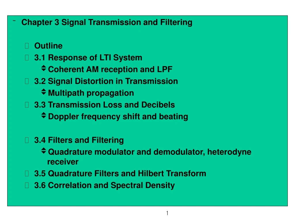
Chapter3 Signal Transmission and Filtering • Outline • 3.1 Response of LTI System • Coherent AM reception and LPF • 3.2 Signal Distortion in Transmission • Multipath propagation • 3.3 Transmission Loss and Decibels • Doppler frequency shift and beating • 3.4 Filters and Filtering • Quadrature modulator and demodulator, heterodyne receiver • 3.5 Quadrature Filters and Hilbert Transform • 3.6 Correlation and Spectral Density
3.1 RESPONSE OF LTI SYSTEMS • Coherent AM reception and LPF • a system • linear time-invariant system • impulse response and convolution integral • step response • LCCDE and LTI system • transfer function and frequency response • steady-state phasor response • undistorted transmission vs. distorted transmission • block diagram analysis: parallel, serial/cascade, feedback connection
Example 3.3-2 Doppler Shift • beating
3.2 SIGNAL DISTORTION IN TRANSMISSION • Chapter 3 is all about the channel. • 3.1 Heterodyne quadrature modulator and demodulator have LTI filters. • There are 4 types of channels for wireless communication using EM wave in the RF band .
If interference and noise are ignored; • The propagation channel is modeled by a linear channel. • Each path has the following four characters: • Gain, Delay • Doppler • Angle/Direction of Departure (AOD/DOD) • Angle/Direction of Arrival (AOA/DOA) • The radio channel maps the propagation channel to a CT SISO/MISO/SIMO/MIMO linear system depending on; • antenna pattern (directivity) and • configurations (spacing). • Directional antenna. Ex. Horn antenna, • Omni-directional antenna • uniform linear array (ULA) • uniform circular array (UCA)
The modulation channel may introduce nonlinear distortion incurred by amplifiers. • The digitalchannel is modeled by a DT system. • Precisely speaking, the channel becomes nonlinear with finite precision. • Often modeled by a linear DT system corrupted by additive quantization noise.
Distortionless Transmission • A channel is distortionless iff it is an LTI system with impulse response • Frequency-flat channel • Overthe desired band • phase • Frequency-selective channel • Distortions • Nonlinear distortions • Linear distortions • Amplitude distortion • Phase distortion
Example: linear distortions Test signal x(t) = cos0t + 1/5 cos50t Figure 3.2-3
Amplitude distortion Test signal with amplitude distortion (a) low frequency attenuated; (b) high frequency attenuated Figure 3.2-4
Phase distortion Test signal with constant phase shift = -90 Figure 3.2-5
Equalization • Multipath distortion • Intersymbol interference (ISI) in digital signal transmission • Linear equalization • Linear zero-forcing equalization (LZF): channel inversion • Linear minimum-mean square error equalization (LMMSE) • Nonlinear equalization • Maximum-likelihood sequence estimator (MLSE) • Decision-feedback equalization (DFE) • Feedforward (FF) filter and feedback (FB) filter • ZF-DFE • MMSE-DFE
CT equalizer vs. DT equalizer vs. block equalizer • Transversal filter, tapped-delay-line equalizer • Frequency-domain equalizer (FDE) • One-tap equalizer for OFDM • Adaptive equalizer • Nonlinear distortion and companding • Transfer characteristic • Memoryless distortion • Distortion with memory • Polynomial approximation of memoryless distortion • Second-harmonic distortion • Intermodulation distortion • Companding • Compressing + expanding
3.3 TRANSMISSION LOSS and DECIBELS • Power gain • g = P_out/P_in • decibels • g_dB = 10 log_10 g • 3 dB = 1/2 • G = 10^(g_dB/10) • Serial interconnection of amplifiers and attenuators -> addition, subtraction in dB • If g = 10^m, then g_dB = m*10 dB • dBm • 0 dBm = 1 mW • 10 dBm = 10 mW • 20 dBm = 100 mW = 0.1 W • 30 dBm = 1 W = 0 dBW
Transmission loss and repeaters • Loss L = 1/g • Path loss • Passive transmission medium • Transmission lines • coaxial cable: Coaxial lines confine virtually all of the electromagnetic wave to the area inside the cable. • Twisted(-wire) pair cable: EMI is cancelled. Invented by A. G. Bell.
Fiber-optic cables • Waveguides • Loss, attenuation • Attenuation coefficient in dB per unit length • Table 3.3-1 • Frequency bands are different. • Fiber optic cable: 0.2-2.5 dB/km loss • Twisted pair: 2-6 dB/km loss • Coaxial cable: 1-6 dB/km loss • Waveguide: 1.5-5 dB/km loss • … • Repeater amplifier • Amplification of distortion, interference, and noise
Optical fiber cable • Total reflection, refraction index Light propagation down a single-mode step-index fiber Figure 3.3-3a Light propagation down a multimode step-index fiber Figure 3.3-3b
Light propagation down a multimode graded-index fiber Figure 3.3-3c
Large bandwidth and low loss • Carrier frequencies in the range of 200 THz • Max bandwidth 20 THz • 0.2-2 dB/km loss • Lower than most twisted-pair and coaxial cable systems • Absorption • Scattering • Less interference • No RF interference • No noise • Low maintenance cost • Secure • Hybrid of electrical and optical components • LED or laser • Envelope detector
Correctionand Announcement • Propagation channel: Each path has gain, … • A channel is distortionless iff it is an LTI system with impulse response • Nonlinear memoryless distortion has input output relation given by which increases bandwidth of the output because multiplication in TD corresponds to convolution in the FD. • Exam on next Tuesday @LG104, 11:00-12:15 • Ch. 1-3 • Open book (but you will not have time to read on the site.) • T/F, filling blanks, Essay, Math
Radio Transmission • Line-of-sight propagation • Free-space path loss (FSPL) • The loss between two isotropic radiators in free space. • Formula • far-field • It is a function of frequency. However, it does not say that free space is a frequency-selective channel.
Example 3.3-1 Satellite repeater system: uplink, downlink, frequency translation, geostationary, low orbit, OBP Figure 3.3-5
3.4 FILTERS and FILTERING • Ideal Filters • LPF • BPF • Lower and upper cutoff frequencies • Passband and stopband • HPF • NF Transfer function of a ideal bandpass filter Figure 3.4-1
Realizability, noncausality • Bandlimiting and timelimiting • It is impossible to have perfect bandlimiting and timelimiting at the same time. Ideal lowpass filter (a) Transfer function (b) Impulse response Figure 3.4-2 Ideal filters are noncausal.
Real-World Filters • Half-power or 3 dB bandwidth • Passband, transition band/region, and stopband Typical amplitude ratio of a real bandpass filter Figure 3.4-3
3.5 QUADRATURE FILTERS and HILBERT TRANSFORMS The quadrature filter is an allpass network that shifts the phase of positive frequencies by -900 and negative frequencies by +900
Example. Hilbert transform of a rectangular pulse (a) Convolution; (b) Result Figure 3.5-2
Instead of separating signals based on frequency content we may want to separate them based on phase content. Hilbert transform Hilbert transform used for describing single sideband (SSB) signals and other bandpass signals
3.6 CORRELATION AND SPECTRAL DENSITY • Stochastic Process = signal with uncertainty described probabilistically Two ways to describe: 1) probability space and mapping to sample path ,2) Kolomgorov’ s extension theorem Non-periodic signal Non-energy signal Ex)Bit Stream Noise Voice Signal
Ensemble Average <At time t> • Correlation • Autocorrelation Function
Time Average vs. Ensemble Average ensemble average time average • Power Spectral Density • Definition. • Theorem.
Interpretation of spectral density functions Figure 3.6-2
Real-Valued Wide-Sense Stationary Processes • Def. A real-valued random process is called WSS if following two properties are met. Property 1. Property 2. 따라서
Power Spectral Density of Real-Valued WSS Random Process (Wiener-Kinchine Theorem) Property 1. Property 2. When X(t) and h(t) are real,
• White Noise 따라서 • Noise : White & Gaussian practically non-white 온도의 함수 “uncorrelated”