Download
1 / 32
320 likes | 524 Views
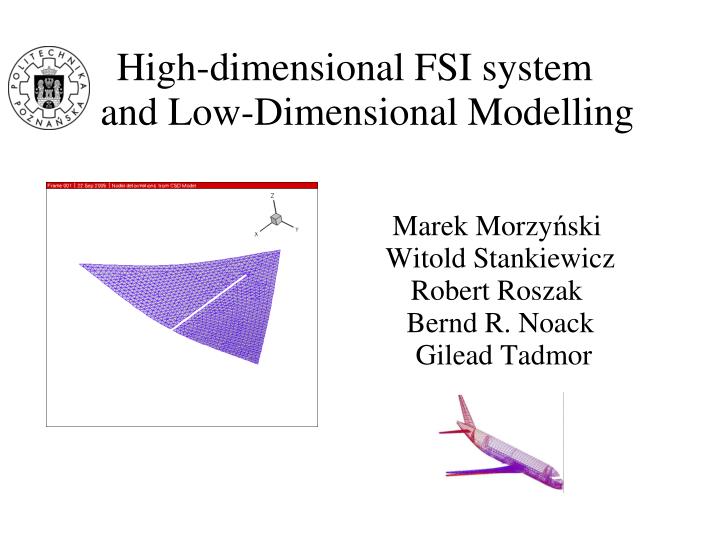
Marek Morzy ń ski Witold Stankiewicz Robert Roszak Bernd R. Noack Gilead Tadmor. High-dimensional FSI system and Low-Dimensional Modelling. Overview. Elements and of High- Dimensional Aeroelastic System Loosely coupled aeroelastic system Computational aspects Elements of the system

E N D
Marek Morzyński Witold Stankiewicz Robert Roszak Bernd R. Noack Gilead Tadmor High-dimensional FSI system and Low-Dimensional Modelling
Overview • Elements and of High- Dimensional Aeroelastic System • Loosely coupled aeroelastic system • Computational aspects • Elements of the system • Solutions • ROM with moving boundaries and ALE • ROM in design and flow control • ROM for AE – sketch of challenges and ideas
ROM AE model - motivation Need of ROM in design AIAA 2008, Rossow, Kroll Need of online capable ROMs in feedback flow control • Aeroservoelasticity • Aeroelastic control • (Piezo-control of flutter, wing • morphing, smart structures) • MicroAerialVehicles • (maneuverability) Aero Data Production A380 wing 50 flight points 100 mass cases 10 a/c configurations 5 maneuvers 20 gusts (gradient lengths) 4 control laws ~20,000,000 simulations Engineering experience for current configurations and technologies ~100,000 simulations
High- Dimensional Aeroelastic System – ROM testbed yes t=t+t convergence Flow code no Tau Code Fluid forces Deformed CFD mesh, velocities Spring analogy Interpolation In-house and AE tools CFD mesh deformation Forces Interpolation MF3 (in-house), Calculix, Nastran Structural code Structure displacements and velocities
Computational aspects – Euler code yes t=t+t Mesh: 10mioelements CPU Power: 16cores convergence Flow code no t=80s Fluid forces Deformed CFD mesh, velocities Interpolation t=10s CFD mesh deformation t=30s Forces Interpolation t=10s Structural code t=4s / 50s Structure displacements and velocities One iteration time: 134s (full CSM) / 180s (modal CSM)
Computational aspects - RANS Mesh: 30mioelements (1 mio: surfaces) CPU Power: 32cores yes t=t+t t=400s convergence Flow code no Fluid forces Deformed CFD mesh, velocities t=90s Interpolation t=220s CFD mesh deformation Forces t=90s t=4s / 50s Interpolation Structural code Structure displacements and velocities One iteration time: 850s (full CSM) / 804s (modal CSM)
High-fidelity CFD and CSM solvers CFD - TAU CODE CSMMF3: in-house CSM Tool • Finite Element-based • Rods, beams, triangles (1st / 2nd order), membranes, shells, tetrahedrons (1st / 2nd order), masses and rigid elements • Static analysis • Transient (Newmark scheme) • Modal analysis • MpCCI and EADS AE interfaces • Finitevolumemethodsolvingthe Euler and Navier-Stokesequations • hybridgrids (tetrahedrons, hexahedrons, prisms and pyramids) • Central orupwind-discretisation of inviscidfluxes • Runge-Kutta time integration • accelerated by multi-grid on agglomerateddual-grids • miscellaneousturbulencemodels • Parallelizedwith MPI • Parallel Chimera grids From DLR TAU-code manual
ALE - Motion of boundary and mesh canonical domain Eulerian approach Lagrangian approach Arbitrary Lagrangian-Eulerian (ALE) bindsthe velocity of the flow u and the velocity of the (deforming) mesh ugrid. For incompressible Navier-Stokes equations the mesh velocity modifies the convective term: With boundary conditions: The fluid mesh can move independently of the fluid particles.
Coupling requirements Alenia SMJ FEM model with 2,815 nodes Alenia SMJ CFD N-S hybrid grid with 1.3 mio nodes and 4.7 mio elements (cells) Aerodynamic mesh 12437 nodes Structural mesh 212 nodes Pressure forces interpolation
Coupling tools Themeshesarenon-conforming • differentdiscretization • differentshape (wholewing/torsionboxonly Non-conservative interpolation Conservative interpolation
Coupling tools • MpCCi (Mesh-based parallel Code Coupling Interface), developed atthe Fraunhofer Institute SCAI • AE Modules, developed in the framework of TAURUS • In-house tools, based on bucket search algorithm AE Modules by EADS and in-house modules perform better in the cases, when only torsion box of the wing was modelled on the structural side.
Dynamic Coupling: time integration General aeroelastic equations of motion : [M] x’’ (t) + [D] x’ (t) + [K] x (t) = f (x, x’, x’’, t) Inertial Damping Elastic Aerodynamic forces forces forces forces Structural forces Newmark direct integration method xi+1 = xi + t xi‘ + t2 [ ( 1/2 - ) xi‘‘ + xi+1‘‘ ] xi+1‘ = xi‘ + t [ ( 1 - ) xi‘‘ + xi+1‘‘ ] Integration in time in CFD (or CSM) code NEWMARK explicit scheme with = 0 and = 0.5 xi+1 = xi + t xi‘ + t2/2 xi‘‘ xi+1‘‘ = ( [M] + t/2 [D] ) -1 { f i+1 - [K] x i+1 - [D] ( xi‘ + t/2 xi‘‘ ) } xi+1‘ = xi‘ + t/2 ( xi‘‘ + xi+1‘‘ )
Fluid mesh deformation • Spring analogy • All edges of tetrahedra are replaced with springs (torsional, semi-torsional, ortho-semi-torsional, ball-vertex, etc.) • The stiffness km of each spring may be constant, or related to element size or distance from boundary • Shephardinterpolation(InverseDistanceWeighting) Based on thedistancesdibetween a givenmeshnode and boundarynodes: • Anotherpossibilities: Elasticmaterialanalogy, VolumeSplines (RadialBasisFunctions), TransfiniteInterpolation
Flutter analysis for I-23 airplane Mach number: M = 0.166, 0.2, 0.3, 044 Atmospheric pressure: P = 0.1 MPa Reynolds number: Re = 2e+6 Angle of attack: α = 0.026 Time step: dt = 0.01 s Singular input function: Fz = 2000 N in time t = 0.01 s
Flutter analysis for I-23 airplane Time history for displacement and rotationincontrolnode on wing Simulation: flutterat Ma=0.44 Experiment: flutterat Ma=0.41
Flutter Laboratory IoA and PUTexperiment and computations • Scale : • Length - 1:4 • Strouhal number 1:1
Experimentalconfigurations • 5 cases – mass added • - 50 grams on the wing's tip • - 20 grams in the middle of ailerons • - 30 grams on vertical stabilizer + 20 grams on tail plane aileron • - 20 grams on horizontal stabilizer • - configuration
FSI - test case 1 • #1 - 50 grams on the wing's tip
Results of test case 1 • #1 - 50 grams on the wing's tip
Low-Dimensional FSI algorithm t=t+t yes Flow ROM convergence no Pressure Deformed CFD mesh, velocities Amplitudes of „mesh” modes Interpolation CFD mesh deformation Forces on structure Interpolation Structural code Structure displacements and velocities
Reduced Order Model of the flow Navier-Stokes Equations 1.GALERKIN APROXIMATION 2. GALERKIN PROJECTION 3. GALERKIN SYSTEM
Projection of convective term ArbitraryLagrangian-EulerianApproach 1.DECOMPOSITION 2. GALERKIN PROJECTION
ROM for a moving boundary NACA-0012 AIRFOIL • 2-D, viscous, incompressible flow • = 15˚, Re = 100 (related to chord length) • displacement of the boundary andmesh velocity: where: T = 5s and Y1 = 1/4 of chord length Inverse Distance Weighted DNS with ALE First 8 POD modes: 99.96% of TKE
ROM for a moving boundary ALE ROM vs DNS Eulerian ROM vs ref. DNS Dumping of oscillationtypical for sub-critical Re The first two modes
AE mode basis for a flow induced by structure deformations • Test-case: bending and pitching LANN wing • Fluid answer to separated, modal deformations (varying amplitudes) • Fluid answer to combined deformation Pressure field and structure deformation(high-dimensional AE) LANN wing structure
ROM AE: CFD → CSM Coupling • We preserve full-dimensional CSM and existing AE coupling tools to interpolate fluid forces on coupling - “wet” - surface; (similarly to Demasi 2008 AIAA) Neighbour search:ae_modules f_cfd2csd Pressure interpolation: ae_modules b_cfd2csd where si (i=1..15) is a distance from CFD node to closest CSM elements • High-dimensional fluid forcesretrived from the Galerkin Approximation
ROM AE: CSM → CFD Coupling and CFD mesh deformation • Linear CSM: deformation decomposed onto mesh modes; Galerkin Projection of ALE term is performed during the construction of GM • Solution of resulting Galerkin System requires only the input of mesh mode amplitudes • Time stepping: the mesh deformation/velocity calculated for next time step with the Newmark scheme ui+1 = ui + t ui‘ + t2[ ( 1/2 - )ui‘‘ + ui+1‘‘ ] ui+1‘= ui‘ + t [ ( 1 - ) ui‘‘ + ui+1‘‘ ]
Mode interpolation Parametrized Mode Basis (Reynolds number here) OPERATING CONDITIONS II POD modes time-avg.solution =0.25 =0.50 shift-mode =0.75 Eigen-modes steady solution M. Morzynski & al.. Notes on Numerical Fluid Mechanics 2007 Tadmor & al. CISM Book 2011 -fast transients OPERATING CONDITIONS I
Results and Conclusions • Advanced platform for FSI ROMs testing open for common research • Computations ongoing • Treatment of CSM - evolution • Linear CSM model • Non-linear CSM model • Tadmor & al. CISM Book 2011 – control capable AE model • Mode parametrization
CFD/CSM • Coupling • Canonical computational domain
Coupling in Low-Dimensional AE • Full-dimensional CSM • The algorithm essentially the same as the high-dimensional one • Interpolation of pressures/forces required • Interpolation of boundary displacements and mesh deformation required: dependent on the chosen approach of boundary motion modelling (acceleration forces / actuation modes / Lagrangian-Eulerian / …) – Tadmor et al., CISM book • Modal CSM • The aerodynamic forces on the surface of structure might be related to the POD (or any other) decomposition of pressure field • Thus: interpolation of pressures/forces not required • Mesh deformation (velocity) modes / actuation modes calculated in relation to the eigenmodes of the structure • The amplitudes of „mesh” modes calculated from the amplitudes of eigenmodes of structure (time integration?) • Thus: interpolation of boundary displacements and mesh deformation not required