Download
1 / 41
410 likes | 527 Views
More LP Formulations. Chapters 5 and 7 McCarl and Spreen. Types of Problem. Joint Product Assembly Disassembly Assembly-Dissassembly. Joint Product. Wool and lamb Trees: Wood, sawdust Grain and straw. Chapter 5: Joint Product. Joint Products Problem Formulation

E N D
More LP Formulations Chapters 5 and 7 McCarl and Spreen
Types of Problem • Joint Product • Assembly • Disassembly • Assembly-Dissassembly
Joint Product • Wool and lamb • Trees: Wood, sawdust • Grain and straw
Chapter 5: Joint Product Joint Products Problem Formulation Basic notation and the decision variable Let us denote the set of : the produced products : the production process possibities : the purchased inputs : the available resources
Joint Product Let us define three fundamental decision variables as : the set of produced product, Sales,product : the set of production possibilities, Production,process : the set of purchased inputs, BuyInput,input
The objective function: We want to maximize total profits across all of the possible productions. To do so, we need to know sale prices of the products, input purchase cost, inputs needed for different production processes, and any other production costs associated with production are needed.
Constraints 1) demand and supply balance for which quantity sold of each product is less than or equal to the quantity yielded by production. 2)demand and supply balance for which quantity purchased of each fixed price input is greater than or equal to the quantity utilized by the production activities. 3) resource availability constraint insuring that the quantity used of each fixed quantity input does not exceed the resource endowments And non-negativity
Algebra Max Subject to
Example: wheat production Two products produced: Wheat and wheat straw Three inputs: Land, fertilizer, seed Seven production processes possible, producing different amounts Of grain and straw and using different amounts of inputs
Other information Wheat price = $4/bushel, wheat straw price =$0.5/bale Fertilizer = $2 per kg, Seed = $0.2/lb. $5 per acre production cost for each process Land = 500 acres
Wheat Production – Solution • 40,000 bushels of wheat and 14,500 bales of straw are produced by 500 acres of the fifth production possibility using 10,000 kilograms of fertilizer and 5,000 lbs. of seed • reduced cost shows a $169.50 cost if the first production possibility is used. • - shadow prices are values of sales, purchase prices of the various outputs and inputs, and land values ($287.5).
The Assembly Problem: Chapter 7 Objective: Maximize the return summed over all the final products produced less the cost of the component parts purchased. Constraints: The first type of constraint equation is a supply‑demand balance and constrains the usage of the component parts to be less than or equal to inventory plus purchases. The second type of constraint limits the resources used in manufacturing final products and purchasing component parts to the exogenous resource endowment. The last type of constraint imposes a minimum sales requirement on final product production
Algebra X is product, Q is component
Example: “Computer Express” Computer Excess (CE) can assemble six different computer types: XT, AT, 80386-25, 80386-33, 80486-SX, and 80486-33. Each different type of computer requires a specific set of component parts. The parts considered: 360K floppy disks, 1.2 Meg floppy disks, 1.44 Meg floppy disks, hard disks, monochrome graphics setups, color graphics setups, plain cases, and fancy cases. Assembly information and resource requirements are given in table 7.1. The resource endowment is 550 hours labor, 240 units of system space and 590 units of shelf space.
Component Parts Information Table 7.1, continued.
Final Products Assembly and Sales Information Table 7.1, continued.
Disassembly: McCarl and Spreen 7 • These problems involve cutting something into parts and selling the parts • Junk yards/salvage operations • Butcher problems • Lumber industry • Some overlap with joint product problem, but emphasis on maximum profit from cutting up a raw products rather than production process
Disassembly Primal, Equations Transforming product to parts Other resource restrictions X indicates the raw product to be cut up into parts and Q indicates the parts. C is the cost of the raw product, d is the sales price of the parts.
Disassembly Objective: The objective function maximizes operating profit, which is the revenue earned by sales of the parts less the costs of all purchased raw products. Constraints: The first constraint is a product balance limiting the quantity sold to be no greater than the quantity supplied when the raw product is disassembled. The next constraint is a resource limitation constraint on raw product disassembly and product sale. The final constraints are upper bounds on disassembly and upper and lower bounds on sales.
Note the typo from the book chapter in red. This number is missing. Jeremiah’s Junk Yard, More Data
More Information on Junkyard • Resource limits: labor, 700 hours; junk yard capacity, 42 units; parts capacity, 60 units. • If its sales limit is reached, chrome is transformed to metal pound per pound. (Note that the upper limit is missing from the table in the book.) • If the sales limit is reached, seats become junk, pound per pound • If the sales limit is reached, doors are transformed to 70% metal, 30% junk
Tableau The easiest way to understand the “convert” activities is to read down the columns – converted seats become junk 1 to 1, converted chrome becomes metal one to one, covert doors are split into metal (70%) and junk (30%).
Scaling Option To get this model to solve properly in Solver, I had to click the option for scaling. If you get a response that says that “conditions for linear model are not satisfied,” click the scaling option and try again. It often clears up the problem. Scaling is useful if coefficients differ greatly in magnitude. (Some programs scale automatically, but Solver does not.)
Assembly-Disassembly, Chapter 7 In this problem, something is broken into parts and then the parts are assembled into new products. Meat packing might be one situation that fits this case. Animals are butchered and cut into parts, which then may be put in packages of different sizes with an assortment of cuts.
General Equations for the Primal X=raw product, Q is manufactured (e.g. assembled) product, T is amount of component parts sold, and Z is the amount of component parts purchased.
Charles Chicken Plucking and Sales Company • Charles Chicken Plucking and Sales Company purchases chickens, cuts them and repacks them. • Chickens cost $1.00 each and have the same weight • Chickens can be cut up several different ways
More Data Table 7.7, continued
Tableau Parts of this problem make more sense if you read down the columns. Note that variable xp to xl all represent chicken purchases, but they are cut in different ways.