Resource Allocation under the Contingency Planning

1. Resource Allocation under the Contingency Planning D. Keselman, Los Alamos National Laboratory

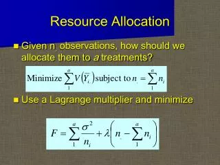
2. Problem Description The problem is to minimize over the set of possible events and possible storage locations the average summary cost of resources, their storage, and transportation to the pre-defined locations, as well as additional penalty cost of not supplying quantities of resources needed at the locations. General formulation is due to W.B. Daniel.

3. Objective function objFun = minWn { minQn {∑l(p(el) * ∑k(∫Ω((pw(l, k, x1k, …, xnk)*∏idxik)   *∑Pm (ps(l, k, π) * minF {CW,X}))))}} CW,X = ∑Ic (c(wi) + ∑k(ck*yik) + ∑k∑Jc(d(wi, sj)*ctk* yik)) + ∑k∑Jck (max{0,  (P(sj) - yijk/ qmink)*cpk}) ∑kVik <= V(wi); Vik <= Ck(wi); ∑Jcyijk <= yik* xik

4. Notation • N – number of candidate buildings to storages. • n – number of storages to be selected. • m – number of consumption points. • D(sj) – demand size of the jth consumption point. • V(wi) – total volumetric capacity of the ith storage. • Vik – limit of volumetric capacity for the kth item in the ith storage. • d(wi, sj) – distance between ith storage and jth consumption point. • Ck(wi) – capacity of ith storage for the item k, Ck(sj) – max demand in the jth demand point.

5. Notation, cont. • c(wi) – cost of maintenance of the corresponding facility. • ck – cost of unit of item k. • ctk – transportation cost of one unit of item k over a distance unit. • s – number of the events under consideration. • el – lth event. • p(el) – probability of event el in a given time span. • pw(l, k, x1k, …, xnk) – combined probability distribution (density function or discrete probability) that after the event l, amount of item k in the warehouses the useable amount will be reduced by the factor xik (0<= xik <=1, i = 1,…, n).

6. Notation, cont. • ps(l, k, π) – probability of a need in item k in the consumption points after the event l, where π represents a vector (α1, …, αm) of 0’s and 1’s with 0 in j position signifies that the jth consumption point has zero demand in the kth item, and 1 represents the opposite. We’ll denote the set of all 2m such vectors by Pm. • cpk – penalty cost coefficient in the objective function incurred by the shortage in item k for one person.  • W – set of all N possible warehouses. • Wn – set of n-element subsets of W.

7. Network Flow Subproblem Cp 1 Wh 1 Sink Source Cp 2 Wh 2 Cp 3 objFun = mean(cost(stored items) + cost(storage maintenance) + cost(delivery) + cost(unsatisfied demand)), objFun –> min

8. Capacities and Costs For source outgoing arcs: capacities – stored item units in a corresponding warehouse, costs – 0. For Wh outgoing arcs: capacities – infinite, costs – trasportation cost of one item unit to a corresponding Cp. For sink incoming arcs: capacities – consumption demands, costs – 0.

9. Algorithm Structure • Preprocessing • Probability combination enumeration • Edge cost sorting • Warehouse combination enumeration • Non-linear optimization • MinCost MaxFlow Batch • Linear Programming

10. Probability Enumeration p1 p2 p3 q1 q2 q3 Assumption: all unusability factor probability distributions are discrete and independent for different warehouses

11. Min Cost Max Flow Batch • Exact • Min Cost Max Flow solution (all combinations) uses Edmonds-Karp algorithm • Approximation • Min Cost Max Flow approximate solution (all combinations) with periodic updates uses a proposition in the next slide and cost edge sorting • Monte-Carlo • Sampling combined distribution

12. Approximation Algorithm Proposition. Let e = (s, w) be a s arc with capacity cap(e) = c, and a maximum flow of minimum cost fMax is equal to f on e: fMax(e) = f. If the capacity of e is changed to c1 with the rest of the network unchanged. Then, c >f and c1≥f implies that fMax is also a maximum flow of minium cost solution in the changed network.

13. Non-Linear Optimization • Simulated annealing • Newton-Raphson method • Gradient descend • Combinatorial brute force

14. Linear Programming Formulation • ∑jwijkl (comb) - wik * xikl(comb) <= 0,   • cjkl(comb) + ∑j wijkl (comb) / qmink >= P(sj),  • wik <= Ck(wi),  • ∑kVik* wik <= V(wi),  • objFun = ∑jklcomb cjkl(comb) * pklcomb) * p(el) * cpk + ∑ik wik* (ck + c(wi)) +  ∑ijklcomb prob ijkl (comb) * p(el) * wijkl (comb) * d(wi, sj) *ctk * sFactorijkl –> min.

15. Some Computational Results Number of Consumption Points = 15

16. Improvements, directions • Improve sampling • Find optimal sampling size as a function of distribution complexity • Use MCMC for higher dimensional problems • Employ multi-commodity flows • Apply LP approach for solving batch flow problems • Expand formulation to mutually interchangeable items