Download
1 / 14
140 likes | 228 Views
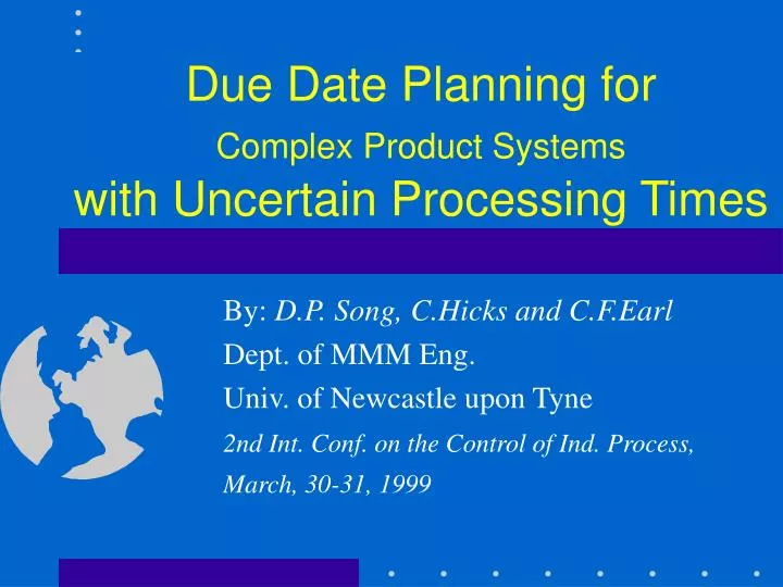
Due Date Planning for Complex Product Systems with Uncertain Processing Times. By: D.P. Song, C.Hicks and C.F.Earl Dept. of MMM Eng. Univ. of Newcastle upon Tyne 2nd Int. Conf. on the Control of Ind. Process, March, 30-31, 1999. Overview. 1. Introduction 2. Literature Review

E N D
Due Date Planning for Complex Product Systemswith Uncertain Processing Times By: D.P. Song,C.Hicks and C.F.Earl Dept. of MMM Eng. Univ. of Newcastle upon Tyne 2nd Int. Conf. on the Control of Ind. Process, March, 30-31, 1999
Overview 1. Introduction 2. Literature Review 3. Simple Two Stage System 4. Leadtime Distribution Estimation 5. Due Date Planning 6. Industrial Case Study 7. Discussion and Further Work
Introduction • Delivery performance • Uncertainties • Complex product system • Assembly • Product structure • Problem : setting due date in complex product systems withuncertainprocessing times
Literature Review Two principal research streams [Cheng(1989), Lawrence(1995), Philipoom(1997)] • Empirical method: based on job characteristics and shop status. Such as: TWK, SLK, NOP, JIQ, JIS • Analytic method: queuing networks, mathematical programming etc.by minimising a cost function Limitation of above research • Both focus on job shop situations • Empirical -- time consuming in stochastic systems • Analytic -- limited to “small” problems
Our approximate procedure • Using analytical/numerical method Þ moments of two stage leadtime Þ approximate distribution Þ decompose into two stages Þ approximate total leadtime Þ set due date
Simple Two Stage System • Product structure Fig. 1 A two stage assembly system
Analytical Result • Cumul. Distr. Func.(CDF) of leadtime W is: FW(t)= 0, t<M1+S1; FW(t) = F1(M1) FZ(t-M1) + F1¢ÄFZ, t ³ M1 + S1. where M1 ¾ minimum assembly time S1 ¾ planned assembly start time F1 ¾ CDF of assembly processing time; FZ¾ CDF of actual assembly start time; FZ(t)= P1n F1i(t-S1i) ľ convolution operator in [M1, t - S1]; F1¢ÄFZ= òF1¢(x) FZ(x-t)dx
Leadtime Distribution Estimation Assumptions • normally distributed processing times • approximate leadtime by normal distr.(Soroush,1999) Approximating leadtime distribution • Compute mean and variance of assembly start time Z and assembly process time Q : mZ, sZ2andmQ, sQ2 • Obtain mean and variance of leadtime W(=Z+Q): mW = mQ+mZ, sW2 = sQ2+sZ2 • Approximate W by normal distribution: N(mW, sW2), t ³ M1+ S1.
Due Date Planning • Mean absolute lateness Þd* = median • Standard deviation lateness Þd* = mean • Asymmetric earliness and tardiness cost Þd* by root finding method • Achieve a service target Þd* by N(0, 1)
Industrial Case Study • Product structure 17 components 17 components Fig. 2 An practical product structure
System parameters setting • normal processing times • at stage 6: m =7days for 32 components, m =3.5 days for the other two. • at other stages : m=28 days • standard deviation: s= 0.1m • backward scheduling based on mean data • planned start time: 0 for 32 components and 3.5 for other two.
Leadtime distribution comparison Fig. 3 Approximation PDF and Simulation histogram of total leadtime
Due date results comparison Table. Due dates to achieve service targets by simulation and approximation methods
Discussion & Further Work • Production plan/Minimum processing times • Skewed distributed processing times • More general distribution to approximate, like l-type distribution • Resource constraint systems