Download

1 / 39
400 likes | 551 Views
This WEEK: Lab: last 1/2 of manuscript due Lab VII Life Table for Human Pop Bring calculator! Will complete Homework 8 in lab Next WEEK: Homework 9 = Pop. Growth Problems Start early!. Chapter 17 Predation + Herbivory. Objectives. Review growth in unlimited environment

E N D
This WEEK:Lab: last 1/2 of manuscript due Lab VII Life Table for Human PopBring calculator! Will complete Homework 8 in labNext WEEK:Homework 9 = Pop. Growth Problems Start early!
Objectives • Review growth in unlimited environment • Geometric growth (seasonal reproduction) • Exponential growth (continuous reprod.) • Population Problems • Growth in limiting environment • Logistic model dN/dt = rN (K - N)/ K • Density-dependent birth and death rates • Assumptions of model • Reality of models
Ch 14: Population Growth + Regulation dN/dt = rN dN/dt = rN(K-N)/K
Two models of population growth with unlimited resources : • Geometric growth: • Individuals added at one time of year (seasonal reproduction) • Exponential growth: • individuals added to population continuously (overlapping generations) • Both assume no age-specific birth /death rates
Geometric growth: > 1 and g > 0 N N0 = 1 and g = 0 < 1 and g < 0 time Growth over 1 time unit: Nt+1 = Nt Growth over many time units: Nt = t N0
exponential growth:dN/dt = rN rate of contribution number change of each of in = individual X individuals population to population in the size growth population
dN / dt = r N • r = difference between per capita birth (b) and per capita death (d) rates • r = (b - d) = # ind./ind./yr
Exponential growth: r > 0 • Growth over many time units: Nt = N0 ert • Doubling time: t2 = ln2/r r = 0 r < 0
The two models describe the same data equally well: ln = r Exponential TIME
How does population size change through time?How does age structure change through time?
How to use a life table to project population size and age structure one time unit later.
Through time • population size increases • fluctuates, then becomes constant • stable age distribution reached
With a stable age distribution, • Each age class grows (or declines) at same rate (). • Population growth rate () stabilizes. • Assumes survival and fecundity = constant.
*** What is a stable age distribution for a population and under what conditions is it reached? • SAD = pop in which the proportions of individuals in the age classes remain constant through time • Population can achieve a SAD only if its age-specific schedule of survival and fecundity rates remains constant through time. • Any change in these will alter the SAD and population growth rate
Populations have the potential to increase rapidly…until balanced by extrinsic factors.
Population growth rate = Intrinsic Population Reduction in growth X size X growth rate rate at dueto crowding N close to 0
Population growth predicted by the logistic model. K = carrying capacity
Assumptions of the exponential model • 1. No resource limits • 2. Population changes as proportion of current population size (∆ per capita) • ∆ x # individuals -->∆ in population; • 3. Constant rate of ∆; constant birth and death rates • 4. All individuals are the same (no age or size structure) 1,2,3 are violated when resources become limited.
Population growth rates become lower aspopulation size increases. • Assumption of constant birth and death rates is violated. • Birth and/or death rates must change as pop. size changes.
Population equilibrium is reached when birth rate= death rate. Those rates can change with density (= density-dependent).
Reproductive variables affected by habitat quality (K is lowered).
r (intrinsic rate of increase) decreases as a linear function of N. • Population growth is density-dependent. rm slope = rm/K r r0 K N
Logistic equation • Describes a population that experiences negative density-dependence. • Population size stabilizes at K, carrying capacity • dN/dt = rmN(K-N)/K, • dN/dt = rmN(1-N/K) • where rm = maximum rate of increase w/o resource limitation = ‘intrinsic rate of increase’ K = carrying capacity • (K-N)/K = environmental break (resistance) = proportion of unused resources
Logistic (sigmoid) growth occurs when the population reaches a resource limit. • Inflection point at K/2 separates accelerating and decelerating phases of population growth; point of most rapid growth
Logistic curve incorporates influences of decreasing per capita growth rate and increasing population size. Specific
Assumptions of logistic model: • Population growth is proportional to the remaining resources (linear response) • All individuals can be represented by an average (no change in age structure) • Continuous resource renewal (constant E) • Instantaneous responses to crowding No time lags. • K and r are specific to particular organisms in a particular environment.
Logistic equation assumes: • Instantaneous feedback of K onto N • If time lags in response --> fluctuation of N around K • Longer lags---> more fluctuation; may crash. N K time
Models with density-dependence: • Built-in time delay ---> can’t continually adjust • Patterns of oscillations depend on value of r (=b-d) >>2 = chaos
Density-dependent factors drive populations toward equilibrium (stable population size), • BUT • they also fluctuate around equilibrium due to: • changes in environmental conditions • chance • intrinsic dynamics of population responses
What controls population size? density-dependent K chance N time density-independent time time
Population dynamics reflect a complex interaction of biotic and abiotic influences, and are rarely stable. Review Ch 15: Temporal and Spatial Dynamics of Populations
Ecological footprints of some nations already exceed available ecological capacity.
Objectives • Review growth in unlimited environment • Geometric growth (seasonal reproduction) • Exponential growth (continuous reprod.) • Population Problems • Growth in limiting environment • Logistic model dN/dt = rN (K - N)/ K • Density-dependent birth and death rates • Assumptions of model • Reality of models