Fundamentals of Electromagnetics with MATLAB Course by Professor Karl E. Lonngren

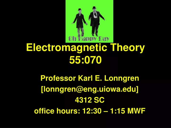
1. Electromagnetic Theory55:070 Professor Karl E. Lonngren [lonngren@eng.uiowa.edu] 4312 SC office hours: 12:30 – 1:15 MWF

2. Demonstration in 2005

3. 207 CC

5. TA: Qiao Hu1313 SC qiao-hu@uiowa.edu Text: “Fundamentals of electromagnetics with MATLAB” 2nd edition/2nd printing SciTech Press Grading 2 exams @ 100 -------- 200 Final exam ---------------- 150 Homework ---------------- 50 Total ----------------------- 400 Arthur Andersen who was recently fired by the Enron Corp. will audit the scores and the addition. Work together?

6. First edition

7. Check the WebSite for this class regularly! -- MATLAB programs -- Old exams Assignments -- Homework solutions -- Scores and Grades

8. Chandra X-ray satellite

9. Crab nebula

10. supernova

11. super bubbles colliding galaxies

12. Ames Ames black hole

13. This is what happens to someone who does not want to learn electromagnetic theory!

15. example • EM Theory • MATLAB & vectors • static em fields • mathematics & MATLAB • Maxwell’s equations • electromagnetic waves & MATLAB • transmission lines & MATLAB • radiation & antennas & MATLAB

16. This course will not be one of those! http://www.jsonline.com/story/index.aspx?id=641947

17. Cash for clunkers

18. MATLAB

19. MATLAB • in the college computers • easy to use & learn • easy to produce 2-d & 3-d plots • ODE & PDE • integrate & differentiate • get pictures – “.m” files in 070 web page • more MATLAB information on the CD

20. >> MATLAB icon >> x = 1 x = 1 >> complex numbers >> y = 1+1j (or 1+ 1i) y = 1.0000 + 1.0000i >> z = x - y z = 0 - 1.0000i >> math

21. >> x = 1; SAVE SPACE TRICK “ ; “ • >> y = 2; • >> z = x * y; % multiply • >> z • z = • 2 • >> w = x / y; % divide • >> w • w = • 0.5000

22. a = 1ux + 2uy + 3uz b = 3ux + 2uy + 1uz c = a + b c = 4ux + 4uy + 4uz >> a = [1 2 3]; >> b = [3 2 1]; >> c = a + b; c = 4 4 4 vectors - addition

23. a = 1ux + 2uy + 3uz b = 3ux + 2uy + 1uz a • b = b • a = 3 + 4 + 3 = 10 >> a = [1 2 3]; >> b = [3 2 1]; >> c = dot(a,b) c = 10 vectors - dot product

24. d = cross (a,b) d = 0 0 1 e = cross (b, a) e = 0 0 -1 vectors - cross product a = 1ux + 0uy + 0uz ==> a = [1 0 0]; b = 0ux + 1uy + 0uz ==> b = [0 1 0];

25. z B - A A B y x |B - A| = norm(B -A)

26. In MATLAB • >>colormap(hot) or cool or  • >>whitebg(‘black’) or ‘green’ or  • “print screen” • “paint”

27. simple graph >> x = [1 2 3 4 5] x= 1 2 3 4 5 >> plot(x) >> xlabel(‘#’) >> ylabel(‘value’)

28. semicolon two values >>x=[1 2 3 4 5]; >>y=[5 4 3 2 1]; >>plot(x,y,’*’) >>xlabel(‘x’) >>ylabel(‘y’)

29. Add to the graph • clear;clf • x=0:.1:4*pi; • plot(sin(x),'linewidth',3) • hold on • plot(cos(x),'linewidth',3,'linestyle','--') • xlabel('x','fontsize',18) • ylabel('V','fontsize',18) • set(gca,'fontsize',18) • whitebg('black')

30. >>[x,y]=meshgrid(-xa : x : xb,-ya : y : yb)

31. >>[x,y]=meshgrid(-1:.1:1,-2:.4:4); >>R=(x.^2+(y+1).^2).^.5; >>Z=(1./R); >>surf(x,y,Z) >>view( - 37.5+ 90, 30)

32. >>[x,y]=meshgrid(-2:.2:2,-2:.2:2); >>r1=(x.^2+(y-.5).^2).^.5; >>r2=(x.^2+(y+.5).^2).^.5; >>V=(1./r1)-(1./r2); >>mesh(x,y,V) >>view(-37.5-90,10) >>colormap(hot)

33. >>[ex,ey]=gradient(V,.2,.2); >>quiver(x,y,ex,ey) >>grid

34. Iterate labels Change styles customize graphs -subplots

35. There are ".m" files on the Web page for this class. -The figures and the examples in the text -Additional programs may be added on an irregular basis

36. Government regulation may be required such as stop signs, stoplights, etc.

38. Babies knows something!