Download
1 / 45
450 likes | 623 Views
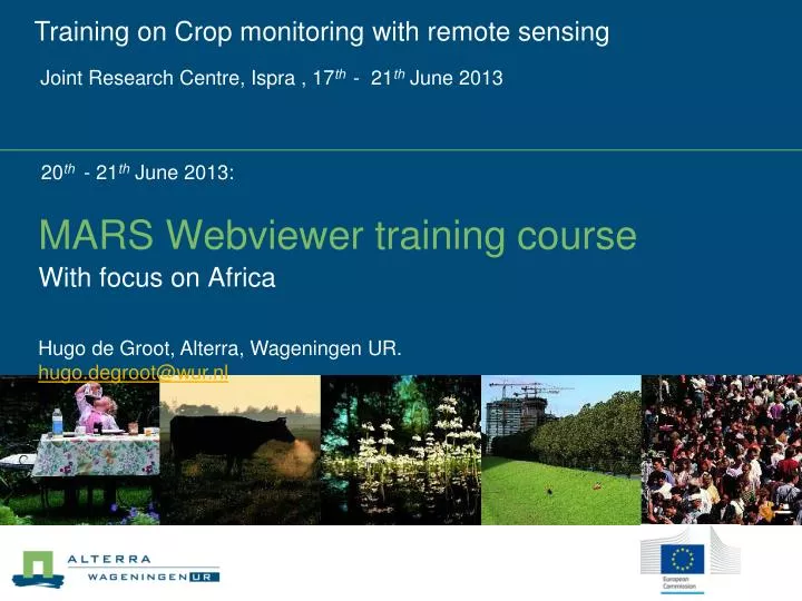
Training on Crop monitoring with remote sensing. Joint Research Centre, Ispra , 17 th - 21 th June 2013. MARS Webviewer training course. 20 th - 21 th June 2013:. With focus on Africa. Hugo de Groot, Alterra, Wageningen UR. hugo.degroot@wur.nl. Content.

E N D
Training on Crop monitoring with remote sensing Joint Research Centre, Ispra , 17th - 21th June 2013 MARS Webviewer training course 20th - 21th June 2013: With focus on Africa Hugo de Groot, Alterra, Wageningen UR. hugo.degroot@wur.nl
Content • Introduction to the MARSOP3 project and data • Exploring MARSOP3 data by using the webviewer • Extensive demo • Hands-on training
MARSOP3: (www.marsop.info) Monitoring Agricultural Resources (MARS)Operational services European Commission JRC: Joint Research Centre IES: Institute for Environment and Sustainability MARS unit (Monitoring Agricultural ResourceS) AGRI4CAST MARSOP3 services FoodSec AGRI-ENV GeoCAP
MARSOP3: list of operational services weather monitoring based on interpolated station data pan-Europe weather monitoring based on ECMWF deterministic forecast pan-Europe and Asia weather monitoring based on ECMWF ensemble models pan-Europe crop monitoring based on interpolated station data pan-Europe crop monitoring based on ECMWF deterministic forecast pan-Europe and Asia crop monitoring based on ECMWF ensemble models pan-Europe crop yield forecast based on interpolated station data pan-Europe crop yield forecast based on ECMWF deterministic forecast pan-Europe and Asia crop yield forecast based on ECMWF ensemble models pan-Europe weather monitoring based on ECMWF deterministic forecast global crop specific drought monitoring global vegetation indices based on SPOT-VEGETATION sensor global vegetation indices based on NOAA-AVHRR sensor global vegetation indices based on METOP-AVHRR sensor pan-Europe vegetation indices based on MODIS-250m sensor pan-Europe and Horn of Africa weather and vegetation indices based on MSG-SEVIRI pan-Europe rainfall estimates based on MSG and observed rainfall Africa
MARS Webviewer MARSOP3 services deliver and store large amounts of basic and added value data (size is now 7 TB !) Basic weather data / Remote Sensing based Vegetation Indices Added value data generated in the various operational levels of the MARSOP3 services through downscaling and aggregation Online viewer enables user to perform spatial and temporal analysis of global state-of-art data sets in a customized way
Exploring the data by using the Mars webviewer http://www.marsop.info Note: Possibility to register (normally access is granted for half a year)
Login to the Mars webviewer guest1 ispra guest2 ispra ... ... ... ... ... guest30 ispra
Choices at startup • Region of interest • Zoom to specific part • Result type • Map, Graph, Quicklook
Viewer capabilities: • Produce MAPS and GRAPHS for spatial and temporal analysis: • On the fly created from the data; based on user choices • Large amount of indicators available • View QUICKLOOKS • Static, preprocessed results from crop monitoring by remote sensing. Indicators: • Normalized Difference Vegetation Index (NDVI) • Dry Matter Productivity (DMV) • Fraction of Absorbed Photosyntheticly Active Radiation (fAPAR) • Rainfall estimates (for whole Africa only)
Map and graph Example of weather indicators Rainfall anomaly april / may
MARSOP: list of operational services weather monitoring based on interpolated station data pan-Europe weather monitoring based on ECMWF deterministic forecast pan-Europe and Asia weather monitoring based on ECMWF ensemble models pan-Europe crop monitoring based on interpolated station data pan-Europe crop monitoring based on ECMWF deterministic forecast pan-Europe and Asia crop monitoring based on ECMWF ensemble models pan-Europe crop yield forecast based on interpolated station data pan-Europe crop yield forecast based on ECMWF deterministic forecast pan-Europe and Asia crop yield forecast based on ECMWF ensemble models pan-Europe weather monitoring based on ECMWF deterministic forecast global crop specific drought monitoring global vegetation indices based on SPOT-VEGETATION sensor global vegetation indices based on NOAA-AVHRR sensor global vegetation indices based on METOP-AVHRR sensor pan-Europe vegetation indices based on MODIS-250m sensor pan-Europe and Horn of Africa weather and vegetation indices based on MSG-SEVIRI pan-Europe rainfall estimates based on MSG and observed rainfall Africa
Push the button Quicklook: define content User defines which part of the data will be visualized • Hierarchical choices: • Resolution • Theme (service) Indicator • Function • Time period and other additional parameters
Quicklook: view result Possible user actions: = home, start again
Define content: Function Used everywhere Default: Year of Interest (YOI), and default the year of interest is the actual year Other: Long term average (LTA) Difference with long term average Difference with previous year Difference with any other year (availability depends on situation) Important to see the spatial distribution of temporal effects or anomalies ! Demo
Map: map actions Map mode buttons: Activate one, then click inside the map Map action buttons: Perform action immediate on click Additional functionality: Leave this map window, start other part
Push the button Map: define content User defines which part of the data will be visualized • Hierarchical choices: • Resolution • Theme (service) • Crop / Landcover • Indicator • Function • Time period and other additional parameters • Aggregation type
Map: Layers = export or print = home, start again = open additional map window Multiple map windows are linked Demo
Maps and Quicklooks: time out • Hands on: Play around with the viewer in Africa • Change the resolution and view the result map • Change the theme and view the result map • Switch between ‘Quicklooks’ and ‘Maps’ • Change the indicator and view the result map • Play with the function and view the result map • Play with the time period and view the result map • Open multiple linked maps and play around • Go to the ‘Layers’ tab and add additional layers to the map • Don’t change the legend, and don’t look at graphs
Graphs • Always act on at least one ‘spatial entity’, so on a specific area • This ‘spatial entity’ can be of any available resolution • So it can be: • a country (Admin Level 0 = Countries) • a district (Admin Level 1 = Districts) • a grid cell
Graphs: opening a graph • Select a ‘spatial entity’ from the map • Inside the map, activate the ‘Select feature’ tool: • Click inside the map in order to select an area The selected area gets highlighted (maplayer must be visible) • Click on the ‘Add graph window’ button:
Shown before Map: opening a graph = export or print = home, start again = open additional map window Multiple map windows are linked = open graph window for selected spatial entity
Graphs Select the ‘graph type’: Demo
Graph types • All available years • Bar chart • Extra options: • One specific year, one indicator, multiple spatial entities • Line chart, more spatial entities possible (up to 6) • Extra options: and Shift-click ! • One specific year, multiple indicators, one spatial entity • Line chart, more chart series possible (up to 6) • Extra options:
Push the button Graph: define content User defines which part of the data will be visualized • Hierarchical choices: • Theme (service) • Crop / Landcover • Indicator • Function • Time aggregation • Overlapping profile Note: Time period is specified in separate tab
Push the button Graph: define content • Time period: • Default starts at January 1st • Timescale depends on dataset (Theme) • For Africa mostly ‘Dekad’ (10 day periods) • 1 – 10 • 11 – 20 • 21 – end of Month
Define content: Overlapping profile Used for graphs Use: Explore extreme situations Compare with other years Note: The Year of Interest (YOI) is excluded in calculating the overlapping profile values !
Maps and Graphs Maps and Graphs are linked • Functionality at the map window for linking • Select feature tool, works on the ‘active layer’ • The graph gets updated automatically on a change of the selected area (if the selected area is of the same resolution) • The active layer can be changed on the Layers-tab : On a resolution changes the active layer changes automatically Demo
Map and graph Example of remote sensing based vegetation index Indication of green and healthy vegetation cover
Maps and Graphs: time out • Hands on: Play around with maps and graphs in Africa • Open a map window and click the ‘Add graph’ button: • What happens? • Make sure you can open a graph window from the map window • Try the three different graph types, view the graph results • With a graph result on the screen: Change the selected spatial entity by selecting another one from the map • Change the theme, the crop / landcover, the indicator and view the result graphs • Play with the function and the time period and view the result graphs • Play with the overlapping profile and view the result graphs • Switch between ‘Africa’, ‘West Africa’ and ‘Horn of Africa’ • Open multiple linked maps, open a graph from every map window and play around • Go to ‘Home’ and start a graph: graph only window • Question: how to select a ‘spatial entity’
Map legends Each indicator has a default legend, the system legend. Possible user actions: • Edit: Change a legend. • Select: Select a different legend. • Delete: Delete a previous saved legend.
Map legends Edit legend ‘by hand’: • Add / remove legend classes • Change legend class range, color or label
Map legends Legend type: Auto-calculate other than normal legends Class boundaries get calculated on the fly based on the actual values which correspond with the current user choices for variable and time-period. Two types: • Equal area • Equal width
Map legends Show and / or store the result: • Update map = Preview map with the new legend settings. The legend is not yet saved. • Save as = Add this legend to the database storage, for later reuse. It must be stored under a new name. • Save = overwrite this legend with the new settings (only available for an earlier saved legend).
Map legends Select legend: Choose from a selection of legends, designed for this indicator Check ‘Show all’ to choose from all legends:
Map legends Delete legend: Throw away an earlier saved legend Demo
Map legends: time out • Hands on: Play around with legends • Open a map window and view aresult map • Start the legend editor • Add a legend class and view the result map • Remove a legend class and view the result map • Change the color for some classes and view the result map • Play around with the legend types (normal / equal area / equal width) and view the result maps • Save the new legend for later reuse • Did you give the new legend a name? If not, what happened? • Save some more legends • Switch between saved legends and view the result maps • Remove a saved legend
Map viewer Examples: time period: look at growing seasons starting in October or November Go deeper into (and show) aggregation type, within short time period (for Minimum Temperature or so).
Map viewer: Map export facilities • Print • Save as .pdf • Save as .png
Map viewer: export facilities • Print • Save as .pdf • Save as .png • Save as .csv, to open in Excel
Map viewer: Quicklook export facilities After download: • Print from your browser • Save from your browser Demo
Export facilities: time out • Hands on: Play around with the export facilities • Open a quicklook window and view a quicklook result • Download the quicklook • Save the quicklook image on your hard disk • Open a map window and view the result map • Export the result map to your local file system • Open a graph window and view the result graph • Export the result map to your local file system. Try different formats, including .csv • If you have Excel installed: Open the .csv file in Excel