Sections 3-1 & 3-2 Measures of Center

Sections 3-1 & 3-2 Measures of Center

In this chapter, we will revisit the concepts of Center, Variation, and Distribution in more detail. Concepts

∑ means add all values in a set x is a data value n is the number of values in a sample N is the number of values in a population Notation

Definition Measure of Center • Tells you something about the general center of the data. But there are different ways to measure this, which give very different information. • Four Main Measures of Center: • Mean • Median • Mode • Midrange

Arithmetic Mean (usually just called Mean) the average, obtained by adding the values and dividing the total by the number of values Notation sample mean (x-bar) population mean (mu) Definition

Round to one more decimal place than is present in the original set of values. If a number comes out even and you need more decimal places, add 0’s on the end. Even in cases where it seems odd (like having half a person), to be accurate a mean should not be rounded to a whole number. Round-off Rule for Mean, Median, and Midrange

Sometimes, to avoid the effect of extremely high or extremely low values (outliers), we will find a trimmed mean. A percentage is chosen, and we delete that percentage from both the top and the bottom. Then we find the mean of what is left. Trimmed Mean

Find the 5% trimmed mean of the following test scores: 99, 98, 92, 91, 91, 90, 88, 87, 87, 85, 85, 85, 80, 79, 76, 72, 67, 66, 45 Example

Find the 5% trimmed mean of the following test scores: 99, 98, 92, 91, 91, 90, 88, 87, 87, 85, 85, 85, 80, 79, 76, 72, 67, 66, 45 Solution 1. There are 19 scores. Find 5% of 19: 19(0.05) = 0.95, round to 1. 2. Remove the 1 highest and 1 lowest score to get: 98, 92, 91, 91, 90, 88, 87, 87, 85, 85, 85, 80, 79, 76, 72, 67, 66 3. Find the mean of these 17 scores, and the trimmed mean is 83.5.

(w •x) x =  w Weighted Mean A mean in which some values count more than others (many professors use weighting of different categories to figure grades).

Suppose your syllabus states that in this class, Homework is worth 10%, Quizzes are worth 20%, Exams are worth 50%, and the Final is worth 20%. You have the following scores: Homework: total of 130 out of 130 possible points Quizzes, each out of 20: 18, 17, 20, 19, 18, 16 Exams, each out of 100: 78, 75, 72 Final: 104 out of 150 possible Find the weighted mean. Example

First, find the average for each category Homework: total of 130 out of 130 possible points = 100% Quizzes, each out of 20: 18, 17, 20, 19, 18, 16 = 108/120 = 90% Exams, each out of 100: 78, 75, 72 = 225/300 = 75% Final: 104 out of 150 possible = 69.3% Solution

Multiply each category score by what it is worth, divide by total for all weights: It does not matter whether you use the percents as they are, or change them to decimals, as long as you do the same thing when you add up the total for the bottom. Homework is worth 10%, Quizzes are worth 20%, Exams are worth 50%, and the Final is worth 20% So the weighted mean is 79.4, in this case 79.4%. Solution, continued

(f •x) x = n Mean of a Frequency Distribution A mean of a frequency distribution is similar to a weighted mean. It can be estimated by using the midpoint of a class as the value for each item in that class.

Suppose you are given the following frequency distribution for the ages of members in a particular social club. You are not given the original data. Estimate the mean age. Age Frequency 20-29 4 30-39 8 40-49 9 50-59 7 Example

To estimate the mean age, start by finding the midpoint of each class. Also find the total frequency. Age Midpoint Frequency 20-29 24.5 4 30-39 34.5 8 40-49 44.5 9 50-59 54.5 7 Total Frequency = 28 Solution

Now as an estimate, we can assume that each person in a class has the midpoint age, and use this to find the mean. Age Midpoint Frequency 20-2924.5 4 24.5(4 people) = 98 30-3934.5 8 34.5(8 people) = 276 40-4944.5 9 44.5(9 people) = 400.5 50-5954.5 7 54.5(7 people) = 381.5 Total Frequency = 28 Total Age = 1156 Estimated mean age = 1156  28 ≈ 41.3 years old Solution, Continued

Median the center when the data values are put in order denoted by x (pronounced ‘x-tilde’) is not affected by an extreme value the way a mean can be Definitions ~

Finding the Median If you have an odd number of values, take the one in the middle If you have an even number of values, average the two in the middle

1.Find the median for the test scores: 86, 52, 73, 82, 79 Put them in order: 52, 73, 79, 82, 86 *Odd number of values, so the median is the one in the middle: 79 Round one decimal place further than the originals, so 79.0 2.Find the median for the test scores:100, 99, 98, 92, 91, 91, 90, 88, 87, 87, 85, 85, 85, 80, 79, 76, 72, 67, 66, 45 *An even number of values (20), so the median is the average of the middle two (the 10th and 11th): (87 + 85) / 2 = 86.0 Examples

First we will talk about entering data into the calculator. Then we will use the calculator to put data in order (in case it is given to you all mixed up), which is helpful for finding the median or a trimmed mean. Then we will be using a function in your calculator to find the mean and median (and eventually lots of other stuff) without even having to sort the list. For the examples, let’s use these test scores: 86, 52, 73, 82, 79 Calculator: TI–83or TI-84

Press STAT Choose 1: Edit Enter the list of data values under L1 CalculatorEnter Data

Press STAT Choose 2: SortA( This sorts in Ascending order Enter the list you want it to sort L1 is 2nd, 1; L2 is 2nd, 2; etc. Go back to STAT, 1: Edit Look at your list—it is now sorted. CalculatorPutting Data in Order

Press STAT Arrow over to CALC Select 1:1-Var Stats A screen will pop up that says 1-Var Stats and has a blinking cursor at the end of it. It is waiting for you to clarify which set of data or list. If your data is all under L1, you can just hit ENTER now.If you put your data under a different column, you need to type in which list before hitting enter. (L2 is the 2nd2, etc.) Calculator1-Var Stats OR

1-Var Stats 1-Var Stats will give you a screen that looks somewhat like this. You can hit the down arrow to see more information. There are three important values for now. is the sample mean, n is the number of data values you entered. Use the down arrow to see more statistics. Toward the bottom, Med is the median. Note that the calculator does not round correctly, but you should. You should be able to find these values by hand and on the calculator.

Press STAT, 1: Edit Enter the class midpoints under L1 and the frequencies under L2 Press STAT, CALC Select 1:1-Var Stats You need to tell it to use both columns. Type L1 (2nd 1), then press the comma button (over the 7), then type L2 (2nd 2), then ENTER. 1-Var Stats for Frequency Distributions OR

Midrange the value midway between the highest and lowest values in the original data set highest score + lowest score Midrange= 2 Definitions

Mode The value that occurs most in the list denoted by M The mode is not always unique. You can have one, two (bimodal), or more. If there is a tie for the value that occurs most often, then the mode is a list of all values in the tie. If none of the values repeat, there is NO mode. For a frequency distribution, the mode would be the class with the highest frequency. Definitions

The distribution is the shape when a frequency distribution or other data is represented visually. (Histogram, polygon, etc.) Symmetric Data is symmetric if the left half of its histogram is roughly a mirror image of its right half. (Need not be perfect.) Skewed Data is skewed if it is not symmetric and if it extends more to one side than the other. Distributions

Distributions

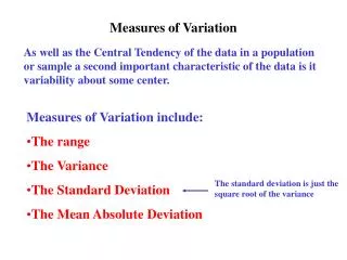
Section 3-3 Measures of Variation

In the next slide, imagine waiting in line at two different banks. Old Bank has three separate lines, and the next person in each line all have three different wait times. New Bank has one line, with different wait times for the next three people in line.The mean wait times are the same, but which bank would you rather go to? New Bank spreads the wait times out more evenly, so most people would prefer to go there.

Variation Old Bank New Bank 3 min 1 min 4 min 14 min 7 min 7 min

While both banks have the same average wait, at Old Bank you run the risk of picking the line with the 14 minute wait. To avoid this risk, most people would prefer to choose New Bank, because its wait times are more consistent.This shows that measures of center are not the only important issue in analyzing data. We are also interested in consistency, or variation.

Range Standard Deviation Variance Variation is an EXTREMELY important topic in statistics. We will be emphasizing range and standard deviation more than variance. 3 Types of Variation

Like mean and median, all measures of variation get rounded to one decimal place more than the original data values. Round-off Rulefor Measures of Variation

The range is the difference between the highest value and the lowest value Definition Easy to compute, but only gives limited information

Range Old Bank New Bank 3 min 1 min 4 min 14 min 7 min 7 min

Standard Deviation Standard deviation measures how far the different data values tend to be from the mean. We will be finding this on the calculator, not by hand. (Though it can be helpful to look at the formula in the book to see exactly what is happening.) Notation sample standard deviation s population standard deviation σ (sigma)

We will be learning how to find standard deviation on the calculator instead of memorizing formulas. To do this, you are doing the exact same thing you did for finding the mean and median. (See earlier notes for how to do this for a frequency distribution.) STAT, 1: Edit, enter data under L1 STAT  Calc, 1: 1-Var Stats The calculator uses Sx to stand for s, the sample standard deviation. (But the real symbol is s.) If this is the whole population, look at σx, the calculator’s notation for the population standard deviation. (We rarely use this.) Try this for the sample of 3 times at Old Bank, and then again for New Bank. CalculatorStandard Deviation

Old Bank s = 7.0 min New Bank s = 1.7 min New Bank has a smaller standard deviation, and therefore is the preferable bank to wait in line at. In general, smaller standard deviations are better, because they indicate less variation in values. In other words, we expect values to be close to the mean more often. Results

Things to Remember • Standard deviation measures how spread out the data is—how far the data is from the mean, on average • The value of the standard deviation is usually positive, sometimes 0, and never negative. • Extreme values (outliers) can have a big effect on standard deviation • The units (labels) for standard deviation are the same as the units of the original data values

This rule helps us to make sense out of standard deviation. It states that at least 75% of the data (95% in some cases) is within 2 standard deviations away from the mean. Thus, values farther than that are considered unusual. minimum usual value = mean – 2(standard deviation) maximum usual value = mean + 2(standard deviation) Range Rule of Thumb

We found that New Bank had a mean wait time of 6.0 minutes, with a standard deviation of 1.7 minutes. Find the usual range and interpret it. Example

We found that New Bank had a mean wait time of 6.0 minutes, with a standard deviation of 1.7 minutes. Find the usual range and interpret it. Solution mean + 2(s) = 6.0 + 2(1.7) = 9.4 mean – 2(s) = 6.0 – 2(1.7) = 2.6 We would expect a usual wait at New Bank to be anywhere between 2.6 and 9.4 minutes.

Definition Empirical Rule For data sets having a symmetrical, bell-shaped distribution, we can be even more specific about percentages that fall within certain ranges. About 68% of all values fall within 1 standard deviation of the mean About 95% of all values fall within 2 standard deviations of the mean (This is the one we use the most!) About 99.7% of all values fall within 3 standard deviations of the mean

The Empirical Rule

The Empirical Rule 2.35% 2.35% 0.15% 0.15%

Sample Population Definition The coefficient of variation (or CV) for a set of sample or population data, expressed as a percent, describes the standard deviation relative to the mean. This tells you what percent of the mean the standard deviation is.

Sections 3-1 & 3-2 Measures of Center