Performance & Stability Analysis

1. Performance & Stability Analysis Professor Walter W. Olson Department of Mechanical, Industrial and Manufacturing Engineering University of Toledo

2. Outline of Today’s Lecture • Review • Two mathematical problems in controls • roots • trajectories • Numerical Methods • Newton Raphson • RungeKutta • System Response • Hypothetical but common 2ne Order System Response • Stability • Determining Stability

3. Two Mathematical Problems Frequently Encountered in Controls • Find the roots of an equation • Methods • Trial and Error (bracketing methods add a bit of science to this) • Graphics • Closed form solutions (e.g.: quadratic formula) • Newton Raphson • Find the solution at a given time for given conditions • Various differential and difference equations analytic solutions (sometimes reformulated as find the roots problem) • Numerical Methods • Newton Cotes Methods (trapezoidal rule, Simpson’s rule. etc. for integration) • Euler’s Method • RungaKutta/Butcher Methods • Many other techniques (Adams-Bashforth, Adams-Milne, Hermite–Obreschkoff, Fehlberg, Conjugate Gradient Methods, etc.)

4. Numerical Methods • Solutions can be approximated using numerical methods • Why Numerical Methods? • Analytical methods may not exist to solve for the exact roots or the exact solution • Use of computers • Flexibility of making changes

5. Newton Raphson Method for finding roots • Probably the most common numerical technique • simple • efficient • flexible • It can be shown from a truncated Taylor’s Series that • Provided that the slope at the test points is consistent, we can iterate to a solution within our error tolerance f(t) f(ti) ti+1 ti Problems occur if the slope reverses sign such as in an oscillation or becomes very flat t

6. Solution Methods • To solve We can use • Reduction in order • Undetermined coefficients • Variation of parameters • Laplace Transforms • Superposition of particular integrals • Cauchy-Euler equation • Numerical methods

7. Euler Method Prediction yi • Our goal is to solve equations of the form • The theory for the Euler method is the same as that of the Newton Raphson Method: • Rather than now solve for an axis crossing, we predict where the next value of the curve will be and then • Make successive estimates of yi+1 yi+1 } Error xi xi+1 } step h

8. RungeKutta/Butcher Method • Has its origins in a 2 variable Taylor Series Expansion • The function is called the increment function • RK4 is a four factor expansion of the incrementing function • For RK4: • Butcher’s method uses 5 factors is more accurate than RK4 at a given time step

9. Hypothetical (but Common Form) 2nd Order System

10. Hypothetical (but Common Form) 2nd Order System

11. Hypothetical (but Common Form) 2nd Order System 5 Responses

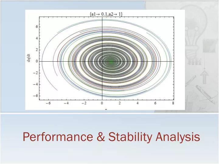
12. Hypothetical (but Common Form) 2nd Order System 5 Phase Plots Equilibrim Points Limit Cycles

13. 2nd Order System Response z z z

14. System Response: Step Input • The time history of a system’s outputs Often called the system path, trajectory or time series { Overshoot Mp Steady State Rise time, tr Transient period=settling time, ts

15. System Response: Frequency Response • Time history with respect to a sinusoid: Phase Shift, DT Amplitude Ay Amplitude Au Input Sin(t) Period,T Transient Response

16. Types of Common Responses General form of linear time invariant (LTI) system is expressed: The most general form of the response (the solution) is expressed:

17. Definition of Stable • A system described the solution (the response) is stable if that system’s response stay arbitrarily near some value, a, for all of time greater than some value, tf.

18. Unstable Responses

19. Hypothetical (but Common Form) 2nd Order System 5 Phase Plots Unstable Stable Marginally Stable

20. Marginally (Neutrally) Stable • Steady Oscillations are said to be marginally or neurtally stable in the sense of Lyapunov

21. Asymptotically Stable

22. Unstable

23. Summary • Stable System Response • System response to a step • System response to a sinusoid • Hypothetical but common 2ne Order System Response • 5 possible responses • Stability • The ability to remain within a given distance of a value in steady state Next Class: Linear Systems