Download

1 / 39
410 likes | 895 Views
RATIONAL CONSUMER CHOICE. Chapter Outline. The Opportunity Set or Budget Constraint Consumer Preferences The Best Feasible Bundle The Utility Function Approach to Consumer Choice Cardinal Versus Ordinal Utility Using Calculus to Maximize Utility: The Method of Lagrangian Multipliers.

E N D
Chapter Outline • The Opportunity Set or Budget Constraint • Consumer Preferences • The Best Feasible Bundle • The Utility Function Approach to Consumer Choice • Cardinal Versus Ordinal Utility • Using Calculus to Maximize Utility: The Method of Lagrangian Multipliers
Figure 3-1: Two Bundles of Goods • A bundle is a specific combination of goods. • eg. Bundle A = 5 unit of shelter & 7 unit of food
Figure 3-2: The Budget Constraint,or Budget Line • Line B describes the set of all bundles the consumer can purchase of given income & prices. • Its slope is the opportunity cost of an additional unit of shelter • the number of units of food that must be sacrificed in order to purchase 1 additional unit of shelter
Budget Constraint or Budget Line • Suppose consumer’s income M = $100, Price of shelter PS = $5 & Price of food PF = $10 • If the consumer spent all her income on shelter, • she could buy M/PS = 100/5 = 20 • K (20,0) • Horizontal intercept • If the consumer spent all her income on food, • she could buy M/PF = 100/10 = 10 • L (0,10) • Vertical intercept • Budget Constraint - straight line that joins points K & L (Line B)
Budget Constraint or Budget Line • Budget triangle– bounded by budget constraint & the 2 axes. • Feasible setoraffordable set- the bundle on or within the budget triangle • eg. Bundle D (5,4) costs $65 • Bundles that lie outside the budget triangle are infeasible or unaffordable, eg. Bundle E
Budget Constraint or Budget Line • The consumer’s weekly expenditure on shelter & food must add up to her weekly income. • If S & F denote the quantities of shelter & food, the constraint must satisfy: PSS + PFF = M (3.1) • Solve Eq 3.1 for F in terms of S:
Figure 3-3: The Effect of a Risein the Price of Shelter • Price of shelter increased from PS1 = $5 to PS2 = $10 • Vertical intercept remains • Rotates the budget constraint inward
Figure 3-4: The Effect of CuttingIncome by Half • Income M is cut by half from $100 to $50 • horizontal intercept M/PS falls (from 20 to 10) • vertical intercept M/PF falls (10 to 5) • Same slope = - PS/PF = -1/2 • B2 is parallel to the B1
Budgets Involving More Than 2 Goods • Consumer’s choice as between a particular good X & the composite good Y • Composite good the amount of money the consumer spends on numerous goods other than X
Figure 3-5: The Budget Constraints with the Composite Good • For simplicity, the price of a unit of composite good = 1 • if the consumer devotes none of his income to X, he will be able to buy M units of the composite good
Figure 3-6: A Quantity Discount Gives Rise to a Nonlinear Budget Constraint • Budget constraint straight line when relative prices are constant - the opportunity cost of one good in term of any other is the same • Budget constraint kinked lines - eg. quantity discounts
Figure 3-7: Budget Constraints Following Theft of Gasoline, Loss of Cash • A theft of $40 worth of gasoline has the same effect on the budget constraint as the loss of $40 in cash. • The bundle chosen should be the same, irrespective of the source of the loss.
Consumer Preferences • Preference ordering a scheme whereby the consumer ranks all possible consumption bundles in order of preference. • Assume world with only 2 goods, the consumer is able to make 1 of the 3 possible statements: • A is preferred to B • B is preferred to A • A & B are equally attractive.
Consumer Preferences • 4 properties of preference orderings: • Completeness • A preference ordering is complete if it enables the consumer to rank all possible combinations of goods • More-Is-Better • Other things equal, more of a good is preferred • Transitivity • For any 3 bundles, if he prefers A to B & prefers B to C, then he always prefers A to C. • Convexity • Mixtures of goods are preferable to extremes
Figure 3-8: Generating EquallyPreferred Bundles • Z > A > W • A = B = C
Z is preferred to A because it has more of each good than A has. • For the same reason, A is preferred to W. • It follows that on the line joining W & Z there must be a bundle B that is equally attractive as A. • In similar fashion, we can find a bundle C that is equally attractive as B.
Figure 3-9: An Indifference Curve • An indifference curve (I) is a set of bundles that the consumer considers equally attractive • L > I > K
Figure 3-10: Part of an Indifference Map • I4 > I3 > I2 > I1
Properties of Indifference Curves • Indifferences curves are ubiquitous. • Any bundle has an indifference curve passing through. • This is assured by the completeness property of preferences. • Indifferences curves are downward-sloping • An upward-sloping I would violate the more-is-better property • Indifferences curves cannot cross • Indifferences curves become less steep as we move downward and to the right along them • This property is implied by the convexity property of preferences
Figure 3-11: Why Two Indifference Curves Do not Cross • E = D (because they lie on the same indifference curve). • D = F (same I) • By transitivity assumption, E = F. But we know that F > E
Figure 3-12: The Marginal Ratesof Substitution • Marginal Rates of Substitution (MRS) • = the rate at which the consumer is willing to exchange the good measured along the vertical axis for the good measured along the horizontal axis • = the absolute value of the slope of the indifference curve (ΔFA/ΔSA)
Figure 3-13: Diminishing MarginalRate of Substitution • The more food the consumer has, the more she is willing to give up to obtain an additional unit of shelter • The convexity property - the consumers like variety
Figure 3-14: People with Different Tastes • Tex is a potato lover; Mohan, rice lover • Tex’s MRS of potatoes for rice is smaller than Mohan’s • Tex willing to exchange 1 potatoes for 1 rice at A • Mohan would trade 2 potatoes for only 1 rice
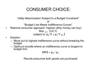
The Best Feasible Bundle • Best affordable bundle - the most preferred bundle of those that are affordable • WHERE is the best affordablebundle located? • the bundle on the budget constraint that lies on the highest attainable indifferent curve • the bundle that lies at tangency between indifference curve & budget constraint
Figure 3-16: A Corner Solution • When the MRS of food for shelter is always < the slope of the budget constraint, the best the consumer can do is to spend all his income on food
Corner Solutions • Corner solution - a case the consumer does not consume one of the goods • Corner solutions occur when goods are perfect substitutes • With perfect substitutes, indifference curves are straight lines, MRS does not diminishing • If MRS steeper than budget constraint, we get a corner solution on the horizontal axis • If MRS less steep, a corner solution on the vertical axis
Figure 3-17: Equilibrium withPerfect Substitutes B = budget constraint
The Utility Function Approach to Consumer Choice • This approach represent the consumer’s preferences with a utility function • A utility function is a formula that yields a number representing the satisfaction provided by a bundle of goods • Eg: U(F,S) = FS, where F = food, S = shelter • if he consume 4 F & 3 S, his utility = 12 • if he consume 3 F & 4 S, his utility = 12
Figure A3-1: Indifference Curves forthe Utility Function U=Fs • To get the indifference curve that corresponds to all bundles that yield a utility level of U0, set FS = U0 and solve for S to get S = U0/F
Figure A3-2: Utility Along an Indifference Curve Remains Constant • Marginal utility (MU) is the rate at which total utility changes as the consumption of goods change • K & L lie on the same indifference curve (same utility) • K L: The loss in utility from having less shelter, MUSΔS = the gain in utility from having more food, MUFΔF
Cardinal Versus Ordinal Utility • Ordinal utility approach • Assumed people are able to rank each possible bundle in order of preference • Does not require that people be able to make quantitative statements about how much they like various bundle • Eg: Able to say prefers A to B, not able to make statement as “A is 6.43 times as good as B” • Cardinal utility approach • The satisfaction provided by any bundle can be assigned a numerical, or cardinal value by a utility function of the form U = U(X,Y)
The Method of Lagrangian Multipliers • We want to find the values of X & Y that produce the highest value of U subject to the constraint that the consumer spend only as much as his income. Maximize £ = U(X,Y) - (PXX + PYY = M) X, Y,
The Method of Lagrangian Multipliers • Taking 1st partial derivatives of £ wrt X, Y & and setting them = 0 • Divide Eq (A.3.9) by Eq (A.3.10)
Example: The Optimal Bundle when U=XY, Px=4, Py=2, and M=40 • Budget constraint is PXX + PYY = M 4X + 2Y = 40 Y = 20 - 2X • U(X,Y) = X(20 - 2X) = 20X - 2X2
Figure A3-6: The Optimal Bundle when U=XY, Px=4, Py=2, and M=40