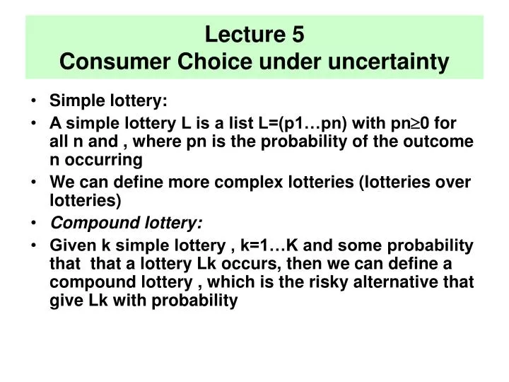
Lecture 5 Consumer Choice under uncertainty

1. Lecture 5Consumer Choice under uncertainty • Simple lottery: • A simple lottery L is a list L=(p1…pn) with pn0 for all n and , where pn is the probability of the outcome n occurring • We can define more complex lotteries (lotteries over lotteries) • Compound lottery: • Given k simple lottery , k=1…K and some probability that that a lottery Lk occurs, then we can define a compound lottery , which is the risky alternative that give Lk with probability

2. Lotteries Example: Prize=100£ Compound lottery A: L1=(100,0,0) occurs with probability 1/3 L2=(100*1/4, 100* 3/8, 100*3/8) with probability 1/3 L3=(=(100*1/4, 100*3/8, 100*3/8) with probability 1/3 Compound lottery B: L1=(100*1/2, 100*1/2, 0) with probability ½ L2=(100*1/2, 0, 100*1/2) with probability ½ Do you prefer A or B?

3. Reduced Lotteries

4. Reduced lotteries • Given all the possible outcomes, we can apply the same logic to compute the probability of each outcome and hence find the Reduced Lottery…

5. Reduced lotteries

6. Preference over compound lotteries Since the consumer only cares about the distribution of final outcomes, he will be indifferent between to Compound Lotteries that deliver the same Reduced Lottery Do you agree?

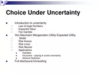
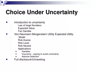
7. Preferences over lotteries • Remember when we defined preferences over a set of goods…. • Again now we have to define preferences but over a space of lotteries - AXIOMS • We require: • Continuity - given two lotteries, small changes in probabilities do not change the ordering between two lotteries • Indipendence: if we mix each of the two lotteries with a third one, the preference ordering of the two resulting mixtures does not depend on the particular third lottery that is used. • Note the difference with the consumer choice under certainty: here when we consider three alternative lotteries L1, L2 and L3, the consumer cannot consumer L1 and L2 together or L1 and L3 together etc. but he has to choose between mutually exclusive alternatives!

8. Expected Utility

9. Expected Utility • Expected Utility theorem • If preferences over lotteries satisfy the continuity and the independence axioms, then preferences can be represented by a utility function with expected utility form • Indifference curves • Since the Von-Neuman-Morgestern utility is linear in probabilities, if we represent the indifference curves on the lottery space, we will obtain parallel straight lines • If not straight lines: indipendence axiom not satisfied **** • If not parallel: indipendence axiom not satisfied ****

10. Consumer choice under uncertainty • If preferences admit expected utility form representation, then the consumer choice under uncertainty reduces to the maximisation of his expected utility, given his budget constraint

11. Money Lottery and risk adversion • Solving problems under uncertainty we can see that individuals show some degree of risk aversion • Where does risk aversion come from? • In other words, which property of the utility function in the expected utility framework implies risk aversion? • Suppose that we define utility over monetary lotteries. Let x be certain amount of money an individual receives • And u(x) the utility associated x. We can show that risk aversion is implies by CONCAVITY of u(x).UNIQUENESS • Is the utility function unique? • NO - - ANY MONOTONIC TRANSFORMATION REPRESENTS THE SAME PREFERENCES • UTILITY IS AN ORDINAL CONCEPT NOT A CARDINAL CONCEPT!

12. Utility function Risk aversion Concave utility function

13. Utility function

14. Risk Aversion • Risk aversion can also be seen using two other concepts: • Certainty equivalent = the sure amount of money that you are willing to accept instead of the lottery • Probability premium = the excess in probability over fair odds that makes an individual indifferent between a certain outcome and a gamble • If an individual is risk averse you expect that: • The sure amount of money he is willing to accept instead of the gamble should be less then the expected value of the money he would get from the gamble (he is willing to take less and avoid the risk) • An individual accepts the risk only if he is offered better than fair odds

15. Measures of Risk Aversion

16. Measures of Risk Aversion

17. Risky Choices Risky choices • Examples of risky choices • Insurance • Investment in risky asset • Comparisons of different payoffs: • Suppose that you are faced with the choice of comparing different risky investments • Which type of statistics about the lottery would you use to choose among investments?

18. Risky Choices • level of return (average) • dispersion of returns • If you know the distribution function, you can use this information to compare lotteries

19. Stochastic dominance • First order stochastic dominance: F(.) first-order stochastically dominates G(.) if:

20. Stochastic dominance • Now, suppose that you can change F(.) in a way that preserves the mean but changes the variance. Suppose that G(.) is the function that you obtain from this transformation, that is G(.) is a mean-preserving spread of F(.) • Ex: F(.) such that with probability p=1/2 you get 2 and with prob p=1/2 you get 3, hence the average payoff is 5/2 • Let be G(.) such that with probability p=1/4 you can get (1,2,3,4) hence the average payoff is again 5/2 • Would you prefer F(.) or G(.)?

21. Stochastic dominance • If you are risk averse, you will prefer F(.) to G(.). • Indeed, we can prove that F(.) second-order stochastically dominates G(.) • Definition • Second order stochastic dominance: given F(.) and G(.) with the same mean, F(.) second-order stochastically dominates (or is less risky than) G(.) if:

22. Stochastic dominance • Result: if G(.) is a mean preserving spread of F(.), then F(.) second-order stochastically dominates G(.) • Proof: • Let x be a lottery distributed according to F(.). Suppose that we further randomize x so that the final payoff is x+z where z is distributed according the the function H(z) with zero mean. Therefore, x+z has the same mean as x but different variance. We define G(.) final reduced lottery, i.e. the function that is assigning a probability to each x using the transformation of F(.) we have just described. Hence G(.) is a mean preserving spread of F(.).

23. Stochastic dominance

24. Expected Utility theory: a calibration exercise Consider the following gamble • You can loose £10 with probability 50% and gain £11 with probability 50% Do you accept this gamble? Consider now these alternative gambles: • Loose £100 with 50% prob. and win 110£ with 50% prob. • Loose £100 with probability 50% and win £221 with 50% prob. • Loose £100 with probability 50% and win £2000 with 50% prob. • Loose £100 with probability 50% and win £20,000 with 50% prob. • Loose £100 with probability 50% and win £1 million with 50% prob. • Loose £100 with probability 50% and win £2 millions with 50% prob. Which bet will you be willing to accept?

25. Source : M. Rabin and R.H.Thaler (2001), Anomalies- Risk Aversion, Journal of Economic Perspectives, pages 219-232

26. Expected Utility theory: a calibration exercise • Problem: the expected utility theory delivers implausible excessive degree of risk aversion!