Download

1 / 15
160 likes | 353 Views
RGB to YUV(CDFG). 林鼎原 Department of Electrical Engineering National Cheng Kung University Tainan, Taiwan, R.O.C. 2012.3.23. v oid main(void) { int a, b, c; ……. RGB_2_Y( I_Frame , O_Frame ); ……. } void RGB_2_Y( I_Frame , O_Frame ); { int y; for ( i =1, i <64, i ++) {

E N D
RGB to YUV(CDFG) 林鼎原 Department of Electrical Engineering National Cheng Kung University Tainan, Taiwan, R.O.C 2012.3.23
void main(void) { int a, b, c; ……. RGB_2_Y(I_Frame, O_Frame); ……. } void RGB_2_Y(I_Frame, O_Frame); { int y; for (i=1, i<64, i++) { y=0.257*a +0.504*b+0.098*c+16; write(y) to O_Frame;} }
Simple Operation description • Y=0.257a +0.504 b +0.098 c +16 • i=1----------------------------------------------------------(1) L1: If(i>=64) goto L2-----------------------------------------(2) • a=I_P()-----------------------------------------------------(3) • b=I_P()-----------------------------------------------------(4) • c=I_P()-----------------------------------------------------(5) • v1 = 0.257 a---------------------------------------------(6) • v2 = 0.504 b --------------------------------------------(7) • v3 = 0.098 c --------------------------------------------(8) • v4 = v1 + v2 ------------------------------------------------(9) • v5 = v3 + 16 -----------------------------------------------(10) • y = v4 + v5 -----------------------------------------------(11) • O_P()=y----------------------------------------------------(12) • i++ ----------------------------------------------------------(13) • goto L1-----------------------------------------------------(14) L2: Nop----------------------------------------------------------(15)
1 Mux CDFG size i ++ Control line < I_P() I_P() I_P() ← ← ← a b c 0.257 0.504 0.098 * * * v3 v1 16 v2 + + v5 v4 + y ← O_P()
Simple Operation description(resource) • Y=(0.257a +16)+0.504 b +0.098 c • i=1----------------------------------------------------------(1) L1: If(i>=64) goto L2-----------------------------------------(2) • a=I_P()-----------------------------------------------------(3) • b=I_P()-----------------------------------------------------(4) • c=I_P()-----------------------------------------------------(5) • v1 = 0.257 a---------------------------------------------(6) • v2 = 0.504 b --------------------------------------------(7) • v3 = 0.098 c --------------------------------------------(8) • v4 = v1 + v2 ------------------------------------------------(9) • v5 = v3 + 16 -----------------------------------------------(10) • y = v4 + v5 -----------------------------------------------(11) • O_P()=y----------------------------------------------------(12) • i++ ----------------------------------------------------------(13) • goto L1-----------------------------------------------------(14) L2: Nop----------------------------------------------------------(15)
Resource constrained 1 Control line system Mux s1 Mux *1 I_P() I_P() I_P() 64 i >= s2 Comparator *1 adder *1 s3 ← ← ← ++ a b 0.257 c multiplexer *1 s4 * 0.504 s5 multiplexer *2 * v1 16 0.098 + multiplexer *2, Adder*1 s6 v2 * v4 + multiplexer *1, Adder*1 s7 v5 v3 Adder*1 s8 + y 資源限制下(每單位時間2乘1加) 需花費8個cycle完成。 ← O_P()
Time –Constrained Scheduling 1 system Mux s1 Mux *1 I_P() I_P() I_P() 64 i >= s2 Comparator *1 adder *1 s3 ← ← ++ ← a b 0.257 c 0.504 s4 multiplexer *3 0.098 * * * s5 multiplexer *3 16 v3 v1 v2 + Adder*2 s6 + v5 v4 Adder*1 + s7 y ← 時間限制在7個cycle內做完, 代價是需多增加一個乘法器(三個)。 O_P()
Pipelining Schedulingfor 3 Pipeline Latency 1 Mux I_P() s1 I_P() I_P() 64 i s2 >= s3 ++ ← ← ← b a 0.257 c s4 * I_P() I_P() 0.504 I_P() s5 * 0.098 V1 16 s6 ← ← + * ← 0.257 a V2 b c V4 s7 I_P() I_P() I_P() * + 0.504 V3 V5 s8 + * 0.098 V1 y 16 ← ← ← s9 0.257 + a * ← V2 b c V4 s10 * O_P() 0.504 + s11 V3 V5 * + 0.098 V1 16 y s12 + * ← V2 V4 s13 O_P() + s14 V3 + 沒pipeline時,相同指令做三次總共需8*3=24個cycle 而有pipeline(3個Latency),總共花費8+(3-1)*3=14個cycle, 節省了4個cycle。 V5 y ← O_P()
Loop Body of 3 Pipeline Latency 2registers 1 adders 2 multipliers Reg數目 * a 2 V2 V3 0.257 c5 s1 + * b 2 V4 V5 0.504 c1 + c6 s2 * c 2 V6 V1 16 c2 0.098 s3 + c3 y * c4 2 V3 V2
Left edge algorithm to allocate values into registers Lifetimes of Values
Lifetimes of Operations * * * * + * * + + + + +
IPData Path Generation R1= {V1, V3, V5} R2= {V2, V4,V6} 0.257 R2 R1 0.504 0.098 b c a 16 1 3 2 1 1 3 3 2 2 3 1 2 M1 M2 M4 M3 * +
Data Path Optimization R1= {V1, V3, V5} R2= {V2, V4,V6} 1, 2, 3 0.257 R2 R1 0.504 0.098 b c a 16 1 3 2 1 3 2 3 1, 2 M1 M2 M3 * + 1, 2, 3
IPController Design R1.ena = R2.ena = State1 + State2 + State3 M1.s1 = M2.s1 = M3.s = State3 M1.s0 = M2.s0 = State2 S0: reset S1:接收input data a ,並運算 a*0.257, V2+V3 S2:接收input data b ,並運算 b*0.504, V4+V5 S3:接收input data c ,並運算 c*0.098, V1+16 , 每次做完counter都會累加1,若counter<64,則回到S1重複做。 S0 S1 S2 S3 reset
Simple Controller Mux Control signals from data path or ROM INCR 累加器 Program counter 計數器 Jump address Microcode ROM Mode Registers …. Control lines Control lines