Parent-offspring conflict… A parent would maximize its fitness by producing as many

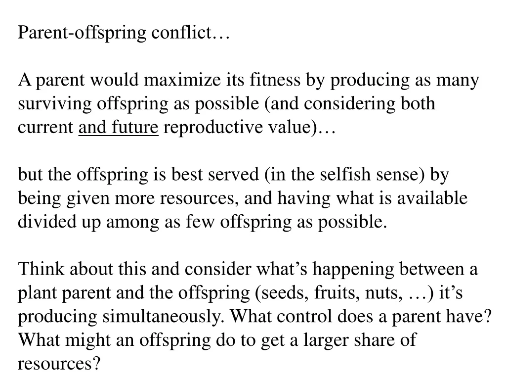
1. Parent-offspring conflict… A parent would maximize its fitness by producing as many surviving offspring as possible (and considering both current and future reproductive value)… but the offspring is best served (in the selfish sense) by being given more resources, and having what is available divided up among as few offspring as possible. Think about this and consider what’s happening between a plant parent and the offspring (seeds, fruits, nuts, …) it’s producing simultaneously. What control does a parent have? What might an offspring do to get a larger share of resources?

2. Readings for lectures today and Tuesday: Chapter 13 pages 256-8 (today) Chapter 14 pages 269-273, 283-289 (today) Chapter 14 remainder (Tuesday) A preliminary form of Tuesday’s lecture is posted with today’s lecture, since you will need it to answer some of the problems for next week’s lab. It will (almost certainly) be modified before Tuesday.

3. Populations Population can be defined in two ways to serve the needs of ecology... One is ecological in context: “A population is comprised of individuals of a single species that occupy the same general area, rely on the same resources, have a high likelihood of interacting with one another, and are influenced by similar environmental factors.”

4. The second is genetic in context, but also important in ecology: “A population is a group of individuals living in close enough proximity to have both the potential to interbreed (conspecifics) and a reasonable likelihood of that occurring.”

5. A population has properties – some are characteristics that can be assessed in individuals, and some have meaning only for the population as a unit. Individual properties: a life history (how long it takes to mature, how frequently they reproduce, how many young in a litter, how old it is when it dies, …), its size, … Group properties: population size, birth rate, death rate, age distribution, r, dispersion, …

6. In ecology we are interested in distribution and abundance. They depend on a combination of individual and group properties. Considered together, they constitute the population’s structure… First, let’s consider distribution. While there is a continuum of distribution types, there are 3 categories named to represent major patterns. They are: 1) random 2) regular (sometimes called overdispersed or uniform 3) clumped

7. 1) randomly example: trees of any single species in a tropical forest

8. 2)overdispersed (or regularly spaced) examples: penguins establishing territories (why?) tilapia (a tropical lake fish)on nesting territories creosote bushes spaced out by chemical interaction

9. 3) clumped - higher densities where environmental conditions (temperature, light, food, water) are better. This indicates the environment is heterogeneous (and frequently patchy). - this is the most common pattern, especially when populations are viewed from a larger scale perspective.

10. 20 Young-of-the-year perch, forming schools in western Lake Erie represents which type of distribution? • random • regular • clumped • None of these

11. The second area of interest is abundance. We are interested not just in how many there are, but also in the dynamics of the population. How does the size of the population change over time? There are, once more, a continuum of possibilities that are categorized by two “end points”… Density-independent growth …and Density-dependent growth The first models to consider are density-independent

12. In assessing abundance and its dynamics, there are four major factors: B = births (or birth rate) I = immigrants (or immigration rate) D = deaths (or death rate E = emigrants (or emigration rate) The basic equation (a discrete time model): Nt+1 = Nt + B + I - D - E Studies of population dynamics are investigations of one or more of these parameters. Some are harder to quantify than others. Many population models assume that I = E, and drop them from the models.

13. Another simplifying approach in many studies is to assume that over long (ecological) time periods: B + I = D + E If this weren’t the case, we’d either be overrun with species that were growing or seeing a much larger rate of natural extinction for species that were declining. In this initial view, we know when populations will grow… whenever B + I > D + E and that populations will decline… when B + I < D + E

14. We can readily consider a discrete time model of density- Independent population dynamics Consider a population that starts at time T. What is its size at time T+1? At the start, size is N(T) One time unit later, the size is N(T+1) N(T+1) = N(T) + B - D + I – E or, assuming I = E, and converting B and D to per head rates N(T+1)/N(T) =  = (B – D)/N(T) the simplifying symbol  is the difference between birth and death rates (number per head per generation [usually] or some other time interval)

15. The population size at T + 1 (one generation later) is: N(T + 1) =  N(T) Now, what will the population size be at T+2? N(T+2) = N(T+1) = (N(T)) = 2N(T) and at t generations in the future… N(T+t) = tN(T) we normally set the starting time at T=0, so that this reads… N(t) = t N(0) This is the equation describing geometric or exponential growth.

16. The time unit used is usually the generation time for an organism under study that fits the discrete model, and… since there is no indication of any density effect in reducing the number of births or increasing the number of deaths, we are modeling density-independent growth. A parallel model for continuous growth uses the change in size over a time interval (the difference between the number of births and the number of deaths. N/ t = bN - dN b and d are per capita birth and death rates, and (b - d) = r. The result is the familiar equations: dN/dt = rN Nt = N0ert

17. There are important assumptions in these models of density-independent growth… - r (orλ), the per capita growth rate, is a constant* - a population growing exponentially is not limited by resources* - all individuals have identical life histories* - we can ignore complications due to mating, thus we effectively assume reproduction is asexual* (the easiest way is to assume the population is comprised of parthenogenetic females)

18. Other things (beyond assumptions) we recognize about exponential growth: - limits to exponential growth are set by abiotic factors, e.g. weather - the same proportion of population affected by changes in abiotic conditions, whatever its size or density - slope of growth curve (rate of growth) increases as population grows, even though the per capita rate is constant. The slope is determined by both r (or λ), which we assume is constant, and N, the current size of the population, which is increasing

19. How about some examples: Discrete exponential growth: If N(0) = 1000 and the population doubles each generation, (λ = 2), what is the population after 5 generations? N(5) = λ5 (1000) = 32,000 Continuous exponential growth: If r = 0.2 insects/insect/week and N(0) =500, how many insects are there after 20 weeks? N(20) = 500 ert = 500 e(0.2)(20) = 500 e4 = 27,000

20. Typically, small-sized organisms have high values of r. One reason is that small organisms have a short generation time. Here are a few values for r scaled per day: Speciesr Paramecium 1.3 Flour beetle0.12 Rattus 0.015 Dog 0.009 Homo sapiens 0.0003

21. The critical problem for models of exponential growth is… Lack of realism Natural populations are limited by physical and biological features of their environments. These limiting factors prevent exponential growth from continuing for long periods of time. You have seen in Populus simulations a number of different patterns population growth may take. Real populations may show much more ‘complicated’ patterns than the simple models display.

22. Here are real data for heron populations in England, re-drawn after Stafford (1971) -

23. The herons are a useful example that limits to growth are usually evident. Population size varies, but never reaches or exceeds 5000 birds. Models that have a maximum population size, designated by K, also called the carrying capacity, are density-dependent, or logistic models. Here’s what the growth curve looks like:

24. The model tells you what to expect about growth by comparing the current N with the value of K…

25. The logistic model must account for the level of “saturation” of the environment with individuals in the population. For example, if K = 100, and there are currently 50 individuals in a population, we would say that the environment was half saturated with members of this population. (N/K = 50/100 = 50%) At N = 80, the environment is 80% saturated. More important than a value for saturation, as N grows closer to K, the rate of growth within this population should slow.

26. The result of recognizing a carrying capacity, and that growth should slow as the population size increases, is the logistic model… or, re-arranging… This is the logistic equation developed by Verhulst and rediscovered by Pearl and Reed around 1920.

27. This familiar form is the continuous growth model. There is a parallel, discrete form for the logistic. Once more, it calculates the population size for a time one unit later (N.B. not one generation later)… Both the discrete and continuous logistic growth models can be integrated, and the integral is what is usually plotted to give the sigmoid curve. It’s not an easy integration. Here’s the result for the continuous model:

28. The assumptions of the logistic model: 1. r and K are constants, invariant as the population grows – this determines that the effect of increasing number on declining growth rate is linear. 2. the population has a stable age structure (constant proportions of each age group in the population). 3. all individuals in the population have identical life histories – this generally happens only when the individuals are genetically identical. This assumption pretty much eliminates sexual reproduction as a mode for this simple model. 4. there are no time lags in the response of growth rate to density. Implications?

29. 20 Which of the following is not an assumption of the logistic model for population growth? • The population is in a stable age distribution • Individuals in the population have the same schedules for survival and reproduction • Both r and K are constant • Limits to population size are set by abiotic factors

30. Assumption 1 tells us the per head growth rate declines from r when the population ‘begins’ to 0 when the population reaches K. From the equation: When N ~ 0, the per head growth rate is ~ r. When N ~ K, then the per head growth rate is r – r = 0.

31. Assumption 2: When a population has a stable age structure (or distribution), the distribution is called a ‘SAD’. The proportion of the total population in each age class remains constant. As an example, imagine a population of mice comprised of 20 young mice just weaned, 10 sub-adult mice (like teenagers), and 5 adult reproducing mice. If the mice were in a stable age distribution, then when the population had doubled in size we would find 40 young, 20 sub-adults, and 10 reproductive adults.

32. Assumption 4: • “No time lags” means that there is no time interval between the occurrence of an event and its effect on population size or dynamics. • Violations of this assumption: • gestation time lag – an organism is conceived by parents, but its appearance as a separate individual to be counted in the population is delayed by the gestation period. • maturation time lag – the model equation assumes that all countable individuals in a population contribute to growth. Frequently there is a more-or-less extended period of development before reproduction begins.