Optimizing Least Squares Problems Using Numerical Techniques

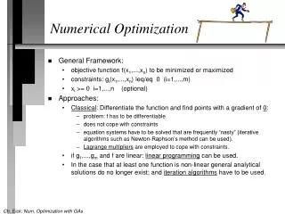
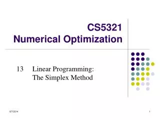
1. CS5321 Numerical Optimization 10 Least Squares Problem

2. Least-squares problems • Linear least-squares problems • QR method • Nonlinear least-squares problems • Gradient and Hessian of nonlinear LSP • Gauss--Newton method • Levenberg--Marquardt method • Methods for large residual problem

3. Example of linear least square • y = β1 + β2x (from Wikipedia) • β1 = 3.5, β2 = 1.4. The line is y = 3.5 + 1.4x

4. T T T T T A A R Q Q R R Q x x y = = Linear least squares problems • A linear least-squares problem is f (x)=1/2||Ax−y||2. • It’s gradient is f (x)=AT(Ax−y) • The optimal solution is at f (x)=0, ATAx=ATy • ATAx = ATy is called the normal equation. • Perform QR decomposition on matrix A = QR. • RT is invertible. The solution x = R−1QTy.

5. m 1 X 2 [ ( ) ] Á t ¡ x y j j ; 2 2 ¡ t ( ) x Á j 1 5 t t t + + + = x x x x x e = 1 2 3 4 ; Example of nonlinear LS • Find (x1,x2,x3,x4,x5) to minimize

6. T 0 0 1 1 ( ( ) ) r m r r x x 1 1 1 X 2 T ( ) ( ) f ( ) ( ) r x r x r x r x = 2 2 j B C B C 2 m ( ( ) ) J R B B C C x x = = X j 1 T = . . B B C C ( ) ( ) ( ) ( ) ( ) f r r J R . . x r x r x x x = = j j @ @ A A . . T ( ) ( ) r r x r x j 1 m m = m X T T 2 2 ( ) ( ) ( ) ( ) ( ) f r J J r + x x x r x r x = j j j 1 = Gradient and Hessian of LSP • The object function of least squares problem is where ri are n variable functions. • Define The Jacobian • Gradient Hessian

7. m 1 1 X m 2 2 T ( ) k k 2 f ( ) ( ) J R f ( ) ( ) ( ) + f r J J x p x r x = X ¼ = x x x T j T 2 2 ( ) ( ) ( ) ( ) ( ) f r J J r 2 2 + x x x r x r x = j j j 1 = j 1 = Gauss-Newton method • Gauss-Newton uses the Hessian approximation • It’s a good approximation if ||R|| is small. • This is the matrix of the normal equation • Usually with the line search technique • Replace with

8. T l J R i 0 m = k k k 1 ! Convergence of Gauss-Newton • Suppose each rj is Lipschitz continuously differentiable in a neighborhood N of {x|f(x)f(x0)} and the Jacobians J(x) satisfy ||J(x)z||||z||. Then the Gauss-Newton method, withk that satisfies the Wolfe conditions, has

9. 2 1 ° ° µ ¶ µ ¶ J 1 R 2 k k ° ° J R i + i + m n p T T m n p ( ) ¸ J J I J R ° p ° + ¡ p 2 ¸ 0 I = 2 p p ° ° ( k k ) ¸ ¢ 0 ¡ p = Levenberg-Marquardt method • Gauss-Newton + trust region • The problem becomes subject to || p ||  k • Optimal condition: (recall that in chap 4) • Equivalent linear least-square problem

10. T µ ¶ k k J T l r J R i 0 k T k m = k ( ) ( ) k k J ¢ i k 0 ¸ ¡ m m p c r m n k k k k k 1 k k T ; 1 k k ! J J k k Convergence of Levenberg-Marquardt • Suppose L={x | f (x)  f (x0)} is bounded and each rj is Lipschitz continuously differentiable in a neighborhood N of L. Assume for each k, the approximation solution pk of the Levenberg-Marquardt method satisfies the inequality for some constant c1>0, and ||pk||k for some >1. Then

11. m X ( ) ( ) ( ) ( ) B r r T T ¡ ¡ 2 2 ( ) ( ) ( ) ( ) ( ) x x r x r x f r J J r = k k k k j j j 1 + 1 + + x x x r x r x = j j j 1 = Large residual problem • When the second term of the Hessian is large • Use quasi-Newton to approximate the second term • The secant equation of 2rj(x) is • The secant equation of the second term and the update formula (next slide)

12. T T T ( ) ( ) ( ) S S S ¡ + ¡ ¡ z s y y z s z s s k k k T S S + ¡ y y = k k m 1 + T T ( ) 2 X y s y s ( ) ( ) ( ) ( ) S B ¡ ¡ x x r x x x = k k k k k k k j ¡ j 1 1 1 1 1 + + + + + s x x = k k 1 + j 1 = T T J J ¡ y r r = k k 1 + k k 1 + m X ( ) [ ( ) ( ) ] r r T T ¡ J J r x r x r x = k ¡ k k j j j 1 1 + + z r r = k k 1 1 + + k k 1 + j 1 = T T J R J R ¡ = k k 1 1 + + k k 1 + Dennis, Gay, Welsch update formula.