Download
1 / 50
500 likes | 552 Views
Digital microscopy: Light Sources and Detectors. Nico Stuurman, UCSF/HHMI UCSF, April 2013. Light Sources. Factors to consider:. Desired Wavelength (Color) Brightness Inherent Brightness Angle!!! Delivery Uniformity (Computer) Control. Brightness is determined by size and angle.

E N D
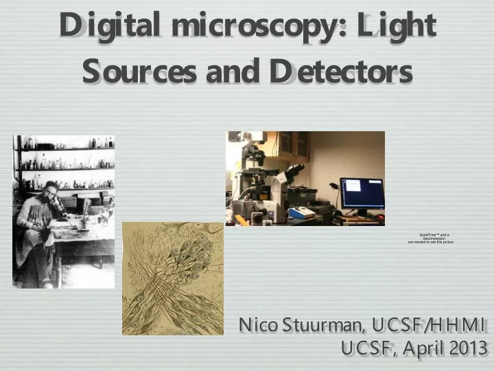
Digital microscopy: Light Sources and Detectors • Nico Stuurman, UCSF/HHMI • UCSF, April 2013
Light Sources Factors to consider: • Desired Wavelength (Color) • Brightness • Inherent Brightness • Angle!!! • Delivery • Uniformity • (Computer) Control Brightness is determined by size and angle
Arc Lamps Mercury Arc Xenon Arc • Cons: • Short Lifetime • Dangerous (Hg) • Hot • Needs mechanical shutter • Laborious installation
Metal Halide Produces light by an electric arc through a gaseous mixture of vaporized mercury and metal halides (compounds of metals with bromine or iodine). • Step up from Arc lamps, still: • Hot, loud, lifetime ~1500 hours • Lamps expensive ($500-800) • Needs mechanical shutter
Source: www.coolled.com White LED with phosphors LEDs Haitz’s law: Every decade the cost per lumen falls a factor of 10, amount of light increases a factor of 20
Lasers Principle Stimulated Emission • Gain Medium • Laser pumping energy • Reflector • Output Coupler • Laser Beam From Wikipedia From Wikipedia Coherent (speckles), Collimated > Dangerous!
Lasers Ion gas Lasers, Argon, Krypton, HeNe • Inefficient > Hot and Loud • No modulation • No longer legal? • Very nice beam quality Argon: 476, 488, 514nm Krypton: 568, 647nm HeNe: 632nm pumped by electric discharge
Lasers Solid-state lasers Optically pumped Laser Diode (electrically pumped) Can be modulated No good yellow (560nm) line? • Highly efficient, small form factor • Some can be electrically modulated • Beam quality good enough
Lasers, coupling Optical Fibers Multi Mode - core > 10 microns Single Mode - core 3-6 micron (visible)
Lasers, modulation • Direct (if possible) • Mechanical shutter • AOM or AOTF • Piezoelectric Optical Device • Switches and modulates intensity • Fast! (sub-microseconds) • Mainly used for excitation laser light • Polarization depended Acousto Optical Tunable Filter Also: AOM or Bragg cell
Imaging Detectors • Detectors: • ‘Single point’ detectors • ‘Multiple point’ detector (cameras)
Single point detector Multi point detector (camera) Lens Detector Camera Analogue Digital Converter (ADC) V time 10 200 35 12 90 85 105 73 80 95 10 200 35 12 90 85 105 73 80 95 Imaging Detectors Photon -> Electrons -> Voltage ->Digital Number Speed! A->V->ADC
Photo-Multiplier Tube (PMT) • Very linear • Very High Gain • Fast response • Poor Quantum efficiency (~25%)
PMT modes • Photon counting mode: • Count pulses • Zero background • Slow • Linear mode • Measure current • Fast but noisy
Avalanche Photo Diode • Absorbed photons->electron • Electrons amplified by high voltage and ‘impact ionization’ • High QE (~90%) • Photon-counting ability (different design) • Overheats if run too fast
… Arrays of photo-sensitive elements
Charged Coupled Devices (CCD) Single read-out amplifier Transfers charge Slow Precise Two Architectures: Complementary Metal Oxide Semiconductor (CMOS) Each pixel has an amplifier Transfers voltage Fast Noisy
CCD Architecture Channel stops define columns of the image Plan View One pixel Three transparent horizontal electrodes define the pixels vertically. Transfer charge during readout Electrode Insulating oxide n-type silicon p-type silicon Cross section
CCD Architecture Electrodes Insulating oxide n-type silicon p-type silicon incoming photons incoming photons
1 2 1 2 3 3 +5V 0V -5V Charge Transfer in a CCD +5V 0V -5V +5V 0V -5V Time-slice shown in diagram
1 2 1 2 3 3 +5V 0V -5V Charge Transfer in a CCD +5V 0V -5V +5V 0V -5V Time-slice shown in diagram
1 2 1 2 3 3 +5V 0V -5V Charge Transfer in a CCD +5V 0V -5V +5V 0V -5V Time-slice shown in diagram
1 2 1 2 3 3 +5V 0V -5V Charge Transfer in a CCD +5V 0V -5V +5V 0V -5V Time-slice shown in diagram
1 2 1 2 3 3 +5V 0V -5V Charge Transfer in a CCD +5V 0V -5V +5V 0V -5V Time-slice shown in diagram
1 2 1 2 3 3 +5V 0V -5V Charge Transfer in a CCD Transfer charge to the next pixel +5V 0V -5V Time-slice shown in diagram
CCD Architectures Mostly EMCCDs Rare Common Full frame CCDs cannot acquire while being read out; They also require a mechanical shutter to prevent smearing during readout.
Why don’t we use color CCDs? • Four monochrome pixels are required to measure one color pixel • Your 5MP digital camera really acquires a 1.25 MP red and blue image and a 2.5 MP green image and uses image processing to reconstruct the true color image at 5 MP
Vital Statistics for CCDs • Pixel size and number • Quantum efficiency: fraction of photons hitting the CCD that are converted to photo-electrons • Full well depth: total number of photo-electrons that can be recorded per pixel • Read noise • Dark current (negligible for most biological applications) • Readout time (calculate from clock rate and array size) • Electron conversion factor (relate digital numbers to electrons)
Pixel size and Resolution 1392 … 1040 … … 6.45 μm on a side … Chip is 8.98 x 6.71 mm Sony Interline Chip ICX285 Typical magnification from sample to camera is roughly objective magnification, so 100x objective -> 65nm per pixel
Resolution and magnification More pixels / resolution element Where is optimum?
Digital Sampling • How many CCD pixels are needed to accurately reproduce the smallest object that can be resolved by the scope? • Nyquist-Shannon Sampling theorem:Must have at least two pixels per resolvable element • 2.5 – 3 is preferable
A resolution-centric view of imaging • Resolution is a function of the objective NA and wavelength (e.g. 1.4 NA with 500 nm light -> ~ 220 nm resolution) • To achieve this resolution, 220 nm in your image must cover 2 pixels • Choose your magnification to achieve this • For 6.45 μm pixels, we need a total magnification of 6450/110 = 58.6 • So for 1.4 NA, a 40x lens would be under-sampled, a 60x would be just at the Nyquist limit, and a 100x lens would oversample
Noise • Longer exposure times are better – why? Decreasing exposure time
Noise • Photon Shot Noise: Due to the fact that photons are particles and collected in integer numbers. Unavoidable! • Scales with √ of the number of photons • Read noise - inherent in reading out CCD • Faster -> Noisier • Independent of number of photons • Fixed Pattern Noise - Not all pixels respond equally! • Scales linearly with signal • Fix by flat-fielding • Dark current – thermal accumulation of electrons • Cooling helps, so negligible for most applications
Signal/Noise Ratio (SNR) • Signal = # of photons = N • Noise = √ (read noise2 + N) • When # of photons << read noise2 -> Read noise dominates • When # of photons >> read noise2-> Shot noise dominates • When shot noise dominates (Signal/Noise = N/√ N), to double your SNR, you need to acquire four times as long (or 2x2 bin)
Often, read-noise dominates 10 photons / pixel on average; ~50 in brightest areas no read noise Test image 5 e- read noise Photon shot noise ~ 3/5 read noise
Binning • Read out 4 pixels as one • Increases SNR by 2x • Decreases read time by 2 or 4x • Decreases resolution by 2x
EMCCD result • Fast noisy CCD – runs at 30 fps, but 50 e- read noise • Multiply signal by 100-fold – now read noise looks like 0.5 e- • Downside – multiplication process adds additional Poisson noise (looks like QE is halved) • Upside – you get to image fast without worrying about read noise
s(cientific)CMOS • < 1.5 electron read-noise! • 2,000 x 2,000 pixels, 6.5 micron • 100 fps full frame, subregions up to 25,000 fps • fixed pattern noise • binning does not reduce r.o. noise • global versus rolling shutter
Dynamic Range: How many intensity levels can you distinguish? • Full well capacity (16 000 e-) • Readout noise: 5e- • Dynamic range: • FWC/readout noise: 3200 • 0.9 * FWC / (3 * readout noise) = 960 • (Human eye ~ 100)
Bitdepth • Digital cameras have a specified bitdepth = number of gray levels they can record • 8-bit → 28 = 256 gray levels • 10-bit → 210 = 1024 gray levels • 12-bit → 212 = 4096 gray levels • 14-bit → 214 = 16384 gray levels • 16-bit → 216 = 65536 gray levels
Measure the electron conversion factor: When the dominant noise source is Photon Shot noise: σ(N)= √(N) Photon Shot noise c = electron conversion factor N = c . DN σ(N) = c . σ(DN) c = DN/σ2(DN) Photons and Numbers • Zero photons collected doesn’t result in number zero. Offset can often be changed • 1 photon does not necessarily equal 1 count in your image – electron conversion factor - depends on camera gain
http://valelab.ucsf.edu/~MM/MMwiki/index.php/Measuring_camera_specificationshttp://valelab.ucsf.edu/~MM/MMwiki/index.php/Measuring_camera_specifications Measure Photon Conversion Factor and full well capacity Photon Transfer Curve from: James R. Janesick, Photon Transfer, DN -> λ. SPIE Press, 2007
Credits and resources: • Kurt Thorn (UCSF Nikon Imaging Center) • http://micro.magnet.fsu.edu • James Pawley, Handbook of Biological Confocal Microscopy • James R. Janesick, Photon Transfer, DN -> λ. SPIE Press, 2007