Inferring phylogenetic trees: Distance methods

1. Inferring phylogenetic trees:Distance methods Prof. William Stafford Noble Department of Genome SciencesDepartment of Computer Science and Engineering University of Washington thabangh@gmail.com

2. One-minute responses • Thank you for this lecture. It was very interesting. • I think I’m starting to program like a pro. • I wish to hear more on how we can understand better the evolutionary relationships among species, preferably among distinct human populations. • I think I enjoyed today’s lecture. More especially the class problems! • 70% of the course has been understood by me. • Tell us more about interpretations. • Python part was easy to follow today. • Python part was very easy to follow. I did not have any problem for the first time. • The lecture was well understood. • The Python part was not so easy for me, but OK. • I appreciate the revision every day, it is very helpful. • Can we learn how to have better output from Python (form / appearance)? • Can we work at this stage on real human genetic data?

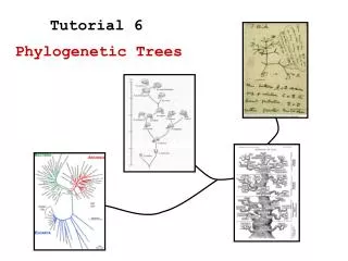
3. Outline • Parsimony • Distance methods • Computing distances • Finding the tree • Maximum likelihood

4. Revision • What is the input to a phylogenetic inference problem? • A multiple alignment of DNA or protein sequences. • What is the output? • A binary tree showing the inferred evolutionary relationships. • For what types of phylogenetic inference problems is maximum parsimony the right approach? • Small numbers of input sequences. • Closely related sequences. • What are the two computational problems that must be solved in a maximum parsimony approach? • Enumerating all possible tree topologies. • Evaluating the parsimony score for a given topology.

5. Revision • Evaluate the parsimony score of the given tree with respect to the first column of the given alignment. Skud Sbay R R Scer Svin R Scer RTGH Skud RTGV Sbay RVGV Smik SVGH Spom STIL Svin RLGH R R R R Score = 1 S S S Smik Spom

6. Revision • Repeat, but use the second column of the alignment. Skud Sbay T V Scer Smik V Scer RTGH Skud RTGV Sbay RVGV Smik SVGH Spom STIL Svin RLGH T X V T T Score = 2 T X L T Svin Spom

7. Selecting a method Choose set of related sequences Obtain multiple sequence alignment Is there strong sequence similarity? Yes Maximum parsimony methods No Is there clearly recognizable sequence similarity Yes Distance methods No Maximum likelihood methods

8. Distance methods Multiple sequence alignment Pairwise distance matrix Phylo- genetic tree

9. Calculating distance ACTGAACGTAACGC Y X Species 2: AATGAAAGAATCGC Species 1: ACTGTAGGAATCGC The distance between species 1 and 2 is the sum of X and Y. Species 1: ACTGTAGGAATCGC Species 2: AATGAAAGAATCGC

10. True evolutionary history Ancestral Species 1 Species 2 A CTGA  C  TA C  GGT  AAA  C  TCGC A C  ATGAAC  AGT  AAA  TCGC  T  C A CTGAACGTAACGC Single substitution Multiple substitutions Coincidental substitutions Parallel substitutions Convergent substitution Back substitution

11. Jukes-Cantor model • Assume the same probability of change at all positions and all times. • dAB is the proportion of changed sites in the alignment. • KAB is the expected number of changes per position. Derivation at http://en.wikipedia.org/wiki/Models_of_DNA_evolution

12. Jukes-Cantor model Species 1 Species 2 3 observed changes in 20 sites A CTGA  C  TA C  GGT  AAA  C  TCGC A C  ATGAAC  AGT  AAA  TCGC  T  C

13. Computing JK distances Proportion of changed sites Species 1: ACGTGATCGGTGA Species 2: ACTTGATGCCTAG Species 3: A-TTACGTAATGG Species 4: A-TTGATGGCGTA Pairwise distances

14. Computing JK distances Proportion of changed sites Species 1: ACGTGATCGGTGA Species 2: ACTTGATGCCTAG Species 3: A-TTACGTAATGG Species 4: A-TTGATGGCGTA Pairwise distances

15. Computing JK distances Proportion of changes sites Species 1: ACGTGATCGGTGA Species 2: ACTTGATGCCTAG Species 3: A-TTACGTAATGG Species 4: A-TTGATGGCGTA From this matrix, we calculate the tree. Pairwise distances

16. Other models • Jukes-Cantor • The simplest possible model • Kimura • 2 parameters • Differentiates between transitions and transversions. • F84, HKY • 5 parameters • Allows arbitrary base frequencies. • Tamura-Nei • 6 parameters • Combination of F84 and HKY. • General time-reversible model • 12 parameters • Only assumes Pr(x→y) = Pr(y→x)

17. Distance methods • Fitch-Margoliash • Neighbor-joining • UPGMA Multiple sequence alignment Pairwise distance matrix Phylo- genetic tree

18. UPGMA • Unweighted pair group method with arithmetic mean. • Also known as agglomerative hierarchical clustering. • Basic idea: iteratively connect the two most closely related sequences.

19. UPGMA

20. UPGMA • Find the smallest off-diagonal element in the matrix.

21. UPGMA • Compute the average between the two rows and columns.

22. UPGMA

23. UPGMA • Each merger creates a subtree. Smik Sbay

24. Perform the next merger Smik Sbay

25. Smik Sbay

26. Smik Sbay Skud Scer

27. What is next? Skud Scer Smik Sbay

28. Formatting with % • Insert % between a string and a tuple to get formatted output. • Use %s for strings, %d for integers, and %f or %g for floats. • Use %f for a fixed number of decimal places, %e for exponent, %g for either. • %g rounds to specified number of digits of precision • %g uses either fixed or exponential notation, depending on the value • Use leading numbers to specify width. • Replace with * to provide width as an input. Full details at http://docs.python.org/2/library/string.html

29. Problem #1 • Write a program that reads sequences from a given file and prints, in aligned columns, the sequence ID, length and frequency of each letter. You may assume that each sequence is no more than 100,000 characters. • Version 1: Use the alphabet ACGT and a fixed width for the sequence ID. • Version 2: Adjust the field width of the sequence ID based on the longest sequence ID. • Version 2: Use the alphabet of the given sequences. Print fields in alphabetical order. • Version 3: Add a header line to your output file. • ./compute-seq-stats.py sample-dna.txt • Read 11 sequences from sample-dna.txt. • ce1cg 77 A=0.17 C=0.12 G=0.31 T=0.40 • ara 87 A=0.34 C=0.23 G=0.18 T=0.24 • bglr1 61 A=0.41 C=0.13 G=0.07 T=0.39 • crp 105 A=0.35 C=0.20 G=0.22 T=0.23 • cya 72 A=0.24 C=0.19 G=0.21 T=0.36 • deop2 102 A=0.29 C=0.11 G=0.25 T=0.34 • gale 73 A=0.30 C=0.23 G=0.12 T=0.34 • ilv 105 A=0.22 C=0.26 G=0.17 T=0.35 • lac 86 A=0.22 C=0.22 G=0.22 T=0.34 • male 54 A=0.31 C=0.24 G=0.28 T=0.17 • malk 65 A=0.26 C=0.15 G=0.37 T=0.22

30. > ./compute-seq-stats-4.py ribosomal.txt Read 13 sequences from ribosomal.txt. Longest sequence ID = 32. 20 letters in alphabet. Alphabet=['A', 'C', 'D', 'E', 'F', 'G', 'H', 'I', 'K', 'L', 'M', 'N', 'P', 'Q', 'R', 'S', 'T', 'V', 'W', 'Y']. Sequence Len A C D E F G H I K L M N P Q R S T V W Y gi|457875803|ref|XP_004224433.1| 108 0.111 0.009 0.009 0.065 0.009 0.028 0.019 0.074 0.194 0.083 0.019 0.046 0.028 0.046 0.028 0.093 0.037 0.065 0.009 0.028 gi|351065825|emb|CCD61804.1 117 0.077 0.009 0.043 0.051 0.009 0.085 0.026 0.026 0.205 0.077 0.017 0.017 0.051 0.026 0.034 0.051 0.043 0.111 0.009 0.034 gi|459660330|gb|EMH75739.1 137 0.146 0.015 0.044 0.044 0.007 0.051 0.015 0.044 0.234 0.066 0.022 0.022 0.066 0.007 0.015 0.058 0.051 0.073 0.015 0.007 gi|449802221|pdb|3ZEY|U 113 0.097 0.018 0.035 0.035 0.018 0.071 0.009 0.044 0.186 0.080 0.044 0.027 0.044 0.035 0.062 0.062 0.053 0.053 0.009 0.018 gi|198419437|ref|XP_002130703.1 112 0.062 0.000 0.027 0.045 0.009 0.071 0.009 0.062 0.179 0.098 0.009 0.036 0.045 0.062 0.054 0.080 0.054 0.054 0.009 0.036 gi|17542024|ref|NP_500895.1 117 0.077 0.009 0.043 0.051 0.009 0.085 0.026 0.026 0.205 0.077 0.017 0.017 0.051 0.026 0.034 0.051 0.043 0.111 0.009 0.034 gi|187129228|ref|NP_001119663.1 116 0.034 0.009 0.043 0.052 0.009 0.078 0.017 0.034 0.216 0.095 0.009 0.017 0.043 0.069 0.043 0.078 0.043 0.078 0.009 0.026 gi|359807542|ref|NP_001241406.1 108 0.102 0.000 0.037 0.028 0.009 0.056 0.009 0.056 0.167 0.074 0.028 0.037 0.065 0.056 0.065 0.102 0.046 0.028 0.009 0.028 gi|351725913|ref|NP_001236341.1 108 0.093 0.000 0.037 0.028 0.009 0.065 0.009 0.056 0.167 0.074 0.037 0.037 0.065 0.046 0.065 0.102 0.046 0.028 0.009 0.028 gi|52346074|ref|NP_001005084.1 125 0.088 0.008 0.072 0.040 0.008 0.072 0.008 0.032 0.216 0.096 0.008 0.048 0.048 0.016 0.048 0.056 0.040 0.064 0.008 0.024 gi|41387126|ref|NP_957109.1 124 0.089 0.000 0.065 0.048 0.008 0.065 0.008 0.032 0.218 0.097 0.008 0.040 0.048 0.024 0.048 0.056 0.040 0.065 0.008 0.032 gi|6323365|ref|NP_013437.1 108 0.139 0.000 0.037 0.046 0.000 0.046 0.028 0.074 0.167 0.083 0.019 0.000 0.037 0.046 0.065 0.093 0.019 0.056 0.009 0.037 gi|6321464|ref|NP_011541.1 108 0.130 0.000 0.037 0.046 0.000 0.046 0.028 0.074 0.167 0.083 0.019 0.000 0.037 0.046 0.065 0.093 0.028 0.056 0.009 0.037