Download
1 / 31
330 likes | 593 Views
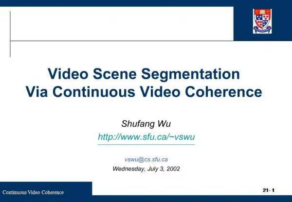
Quantum State Reconstruction via Continuous Measurement. Ivan H. Deutsch, Andrew Silberfarb. University of New Mexico. Poul Jessen, Greg Smith. University of Arizona. Information Physics Group http://info.phys.unm.edu. QUANTUM WORLD. Quantum Information Processing. State Preparation.

E N D
Quantum State Reconstruction via Continuous Measurement Ivan H. Deutsch, Andrew Silberfarb University of New Mexico Poul Jessen, Greg Smith University of Arizona Information Physics Group http://info.phys.unm.edu
QUANTUM WORLD Quantum Information Processing State Preparation Classical Input Control Measurement Classical Output
• State Preparation How well did we prepare ? • Control dynamics How well did we implement a map ? • Sense external fields: Metrology Under what Hamiltonian did the system evolve? Evaluating Performance
Require many copies Quantum State Estimation • Fundamental problem for quantum mechanics: Measure stater Finite dimensional Hilbert space, dim d • Any measurement, at mostlog2dbits/system e.g. Spin 1/2 particle,d=2: one bit. • Density operator, d2-1 real parameters Hermitian matrix with unit trace. • Required fidelity: b(d2-1) bits of information. b bits/matrix-element.
[ ] Tr 1 r = [ ] Re r 12 r 11 + r = r [ ] Im r 12 Stern-Gerlach measurement: Q-Axis Apparatus Observable Information r r ˆ S , z 11 22 [ r ] Re ˆ S 12 x similarly [ r ] Im ˆ 12 S y Note:can equally well rotate system 3 ways & measure Heisenbergpicture density matrix 3 indep. real numbers Spin-1/2:
• Assign probabilities based on sampling ensemble - Standard approach: Strong measurement Each ensemble with possible accuracy of bits Quantum State Reconstruction Basic Requirements: • “Informationally Complete” Measurements
Challenges for Standard Reconstruction Many measurements • Each measurement on ensemble, d-1 independent results. • Require at least d+1 measurements of different observables. Strong backaction • Projective measurements destroy state. • Need to prepare identical ensembles for each Mi Wasted quantum information • Need onlyblog2dbits. Wasteful whenN>>b. • Much more “quantum backaction” than necessary. • Quantum State erased after reconstruction. Alternative -- Continuous measurement
• Ensemble identically coupled to probe (ancilla) Ultimate resolution -- Long averaging “Projection noise” No correlations Continuous Weak Measurement Approach Measurement record Probe noise: Gaussian variance
System Detector Probe Controller Advantages of Continuous Measurement • NMR • Electron transport • Off resonance atom-laser interaction • Weak probes • Real-time feedback control
The Basic Protocol • Continuously measure observable O. • Apply time dependent control to map new information onto O. • Use Bayesian filter to update state-estimate given measurement record. • Optimize information gain.
• Work in Heisenberg Picture (control independent of r0) • Coarse-grain over detector averaging time. Measurement series • Need to generate “complete set” of operators to find Time dependent Hamiltonian, , generatesSU(d) Include decoherence (beyond usual Heisenberg picture) Given find • Stochastic linear estimation: Mathematical Formulation
Conditional probability Single measurement Gaussian Multidimensional Gaussian Least square fit Bayesian Filter Bayesian posterior probability
Optimize Entropy in Gaussian Distribution: = SNR for measurement of observable along principle axisa. Eigenvalues of : full rank Informationally complete Information Gain
Physical System Ensemble of alkali atoms. Total spin F, dim= 2F+1 Measurement: Couple to off-resonant laser Polarization dependent index of refraction: Faraday Rotation q ex = + + - eq = + + eiq- Magnetically polarized atomic cloud Measures average spin projection:
Basic Tool: Off Resonance Atom-Laser Interaction nP3/2 Monochromatic Laser Alkali Atom Hyperfine structure F nS1/2 Tensor Interaction Atomic Polarizability Irreducible decomposition
Irreducible Tensor Decomposition Note: For detunings :
Signal -- Continuous observation of Larmor Precession Larmor Precession AC Stark Shift Photon Scattering Experiment: P.S. Jessen, U of A G. Smith et al. PRL 96, 163602 2004. Collapse and revival of Larmor precession
Enhanced Non-Linearity on Cs D1 Transition Non-linear (tensor) light shift • maximize b µDHF by probing on D1 line - Collapse & revival in Larmor precession (D1 probe) Master Equation Simulation signal [arb. units] Experiment time [ms]
Controlability For magnetic fields alone uncontrollable (algebra closes) The nonlinearity allows full controlability: Our example system effective Hamiltonian: But… Light shift nonlinearity is tied to decoherence.
Measurement Strategy Errors along primary axis given by the eigenvalues ofR 1-1/2 P(0) 2-1/2 P(M|0) • Time dependent B(t) to cover operator space, su(2F+1). Fz • In given trial, system decays due to decoherence. su(2F+1) Maximize information gain in time before decoherence, subject to “costs”
linear polariz. Fix magnitude and Bz=0 B(t) z q Probe (Measure axis) y Choose 50 points along trajectory to specify angles. Interpolate up to full sample rate. - time Quantum State Reconstruction In the Lab: - use NL light shift + time varying B-field to implement required evolution - measure Faraday signal µFz(t)
Spins of 133Cs Some atomic physics 6P3/2 F’ • Off-resonance: 6P1/2 F’ • Scattering rate: D2 D1 • Nonlinear light shift requires detuning not large compared to hyperfine splitting. F=4 6S1/2 F=3 6S1/2 Cesium Doublet 6P1/2 6P3/2 • Scattering time: 1 ms • Detuning: D1 , D2 • Measurement duration: 4 ms • Integration steps: 1000,
Example: D1, F=3, Stretched state 1 .9 .8 .7 .6 .5 Fidelity 50 100 150 200 250 300 350 400 450 500 SNR
Example: D2, F=4, Cat state, 1 .9 .8 .7 .6 .5 .4 .3 Fidelity SNR
fidelity = 0.62 (random guess = 0.38) Quantum State Reconstruction (Cs, F = 3) Preliminary Result Single Measurement Record theory signal (polarization rotation) experiment % error
fidelity = 0.82 (random guess = 0.38) Quantum State Reconstruction (Cs, F = 3) Preliminary Result 128 Average theory signal (polarization rotation) experiment % error systematic errors time [ms]
Inhomogeneities in field intensity - include in model. Optimization naturally seeks “spin-echo” solution. What if control parameters are not known exactly? Background or unknown B-field Assume a distributionP(Bi(t))then
1 Fidelity .7 0 2.5% 1% Robustness to Field Fluctuations Percent error control B-field. Use known state to estimate field and adjust simulation.
Generalized measurements: Ellipticity spectroscopy. F(2) Extensions • Improved optimization (convex sets). • Limited reconstruction: e.g. second moments. • Observation of entangling dynamics. • Toward feedback control of quantum features.
Conclusions • Continuous weak measurement allows quantum state reconstruction using a single ensemble. • Maximizes information gain/disturbance tradeoff. • Can be useful when probes are too noisy for single quantum system strong-measurement but sufficient signal-to-noise can be seen in ensemble. • State-estimation beyond the “Kalman filter”. • New possibilties of quantum feedback control. e-print: quant-ph/0405153, to appear in PRL
http://info.phys.unm.edu/DeutschGroup Trace Tessier Andrew Silberfarb Collin Trail René Stock Iris Rappert Seth Merkel