Download
1 / 93
1.13k likes | 1.76k Views
Introduction to Image Processing. Image Processing. Imaging in the Visible and Infrared Bands. Other Examples. (甲狀腺). Image Sampling and Quantization. Image Sampling and Quantization. S ampling : d igitizing the 2-dimensional spatial coordinate values

E N D
Introduction to Image Processing
Other Examples (甲狀腺)
Image Sampling and Quantization
Sampling: digitizing the 2-dimensional spatial coordinate values Quantization: digitizing the amplitude values (brightness level) Image Sampling and Quantization
PGM file PPM file Representing Digital Images--Examples P2 320 240 255 200 215 25 … 55 25 25… 25 55 255 … P3 # Created by Paint Shop Pro 5 320 240 255 2002152520021525 … 552525 552525 … 25552552555 255 …
Spatial and Gray-Level Resolution Spatial Resolution
8 128 16 256 4 64 32 2 Gray-Level Resolution
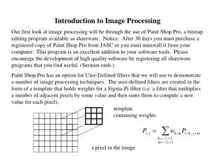
Some Basic Relationships Between Pixels • Pixel Apixel has a location (the spatial coordinate) and a value. • Connected component of S: The set of all pixels in S that are connected to a given pixel in S. • Region of an image • Contour of a region • Edge: Edge is a path of one or more pixels that separate two regions of significantly different gray levels.
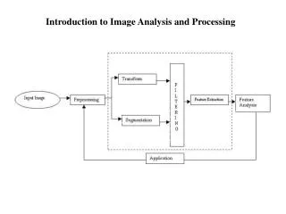
Image Enhancement in the Spatial Domain
A mathematical representation of spatial domainenhancement: where f(x, y): the input image g(x, y): the processed image T: an operator on f, defined over some neighborhood of (x, y) Background
Piecewise-Linear Transformation Functions Case 1: Contrast Stretching
Piecewise-Linear Transformation Functions Case 2:Gray-level Slicing Result of using the transformation in (a) An image
Histogram Equalization • Histogram equalization: • To improve the contrast of an image • To transform an image in such a way that the transformed image has a nearly uniform distribution of pixel values • Transformation function T(r) (continuous case)
Histogram Equalization • In discrete version: • The probability of occurrence of gray level rk in an image is n : the total number of pixels in the image nk : the number of pixels that have gray level rk L : the total number of possible gray levels in the image • The transformation function is • Thus, an output image is obtained by mapping each pixel with level rk in the input image into a corresponding pixel with level sk.
Transformation functions (1) through (4) were obtained form the histograms of the images in Fig 3.17(1), using Eq. (3.3-8). Histogram Equalization
Basics of Spatial Filtering • In spatial filtering (vs. frequency domain filtering), the output image is computed directly by simple calculations on the pixels of the input image. • Spatial filtering can be either linear or non-linear. • For each output pixel, some neighborhood of input pixels is used in the computation. • In general, linear filtering of an image f of size MXN with a filter mask of size mxn is given by where a=(m-1)/2 and b=(n-1)/2 • This concept called convolution. Filter masks are sometimes called convolution masks or convolution kernels.
Smoothing linear filters Averaging filters Box filter Weighted average filter Weighted average Box filter Smoothing Spatial Filters
Smoothing Spatial Filters • The general implementation for filtering an MXN image with a weighted averaging filter of size mxn is given by where a=(m-1)/2 and b=(n-1)/2
Smoothing Spatial Filters Image smoothing with masks of various sizes
Smoothing Spatial Filters Another Example
Order-statistic filters Median filter: to reduce impulse noise (salt-and-pepper noise) Order-Statistic Filters
Image Enhancement in the Frequency Domain
The frequency domain refers to the plane of the two dimensional discrete Fourier transform of an image. The purpose of the Fourier transform is to represent a signal as a linear combination of sinusoidal signals of various frequencies. Background
Introduction to the Fourier Transform and the Frequency Domain • The one-dimensional Fourier transform and its inverse • Fourier transform (continuous case) • Inverse Fourier transform: • The two-dimensional Fourier transform and its inverse • Fourier transform (continuous case) • Inverse Fourier transform:
Introduction to the Fourier Transform and the Frequency Domain • The one-dimensional Fourier transform and its inverse • Fourier transform (discrete case) DTC • Inverse Fourier transform:
Introduction to the Fourier Transform and the Frequency Domain • Since and the fact then discrete Fourier transform can be redefined • Frequency (time) domain: the domain (values of u) over which the values of F(u) range; because u determines the frequency of the components of the transform. • Frequency (time) component: each of the M terms of F(u).
Introduction to the Fourier Transform and the Frequency Domain • The two-dimensional Fourier transform and its inverse • Fourier transform (discrete case) DTC • Inverse Fourier transform: • u, v : the transform or frequency variables • x, y : the spatial or image variables
Introduction to the Fourier Transform and the Frequency Domain • Some properties of Fourier transform:
(a) f(x,y) (b) F(u,y) (c) F(u,v) The Two-Dimensional DFT and Its Inverse • The 2D DFT F(u,v) can be obtained by • taking the 1D DFT of every row of image f(x,y), F(u,y), • taking the 1D DFT of every column of F(u,y)
The Property of Two-Dimensional DFT Rotation DFT DFT
The Property of Two-Dimensional DFT Linear Combination A DFT B DFT 0.25 * A + 0.75 * B DFT
The Property of Two-Dimensional DFT Expansion A DFT B DFT Expanding the original image by a factor of n (n=2), filling the empty new values with zeros, results in the same DFT.
Two-Dimensional DFT with Different Functions Its DFT Sine wave Rectangle Its DFT
Two-Dimensional DFT with Different Functions Its DFT 2D Gaussian function Impulses Its DFT