Download
1 / 57
610 likes | 953 Views
System of Linear Equations. Nattee Niparnan. Linear Equations. Linear Equation. An Equation Represent a straight line Is a “linear equation” in the variable x and y. General form a i a real number that is a coefficient of x i b another number called a constant term.

E N D
System of Linear Equations NatteeNiparnan
Linear Equation • An Equation • Represent a straight line • Is a “linear equation” in the variable x and y. • General form • aia real number that is a coefficient of xi • b another number called a constant term
System of a Linear Equation • A collection of several linear equations • In the same variables • What about • A linear equation • in the variables x1, x2 and x3 • Another equation • in the variables x1, x2,x3 and x4 • Do they form a system of linear equation?
Solution • A linear equation • Has a solution • When • It is called a solution to the system if it is a solution to all equations in the system
Number of Solution • Solution can have • No solution • One solution • Infinite solutions
Example 1 • Show that • For any value of s and t • xi is the solution to the system
Parametric Form • Solution of the system in Equation 1 is described in a parametric form • It is given as a function in parameters s and t • It is called a general solution of the system • Every linear equation system having solutions • Can be written in parametric form
Try another one • Solve it using parametric form • In term of x and z • In term of y and z There are several general solutions
Geometrical Point of View • In the case of 2 variables • Each equation is represent a line in 2D • Every point in the line satisfies the equation • If we have 2 equations • 3 possibilities • Intersect in a point • Intersect as a line • Parallel but not intersect
As a line No intersection As a point
3D Case • What does Ax + By + Cz = D represent?
3D Case • A plane
Higher Space? • Somewhat difficult to imagine • But Linear Algebra will, at least, provides some characteristic for us Cogito, ergo sum I also speak Calculus
Augmented Matrix Augmented matrix Coefficient matrix Constant matrix
Equivalent System System 1 • System a set of linear equations • Two systems having the same solution is said to be “equivalent” • Some system is easier to identify the solution • To solve a system, we manipulate it into an “easy” system that is still equivalent to the original system Solution preserve operation System 2 Solution preserve operation System 3
Elementary Operation Solved!
Elementary Operation • Interchange two equations • Multiply one equation with a nonzero number • Add a multiple of one equation to a different equation
Theorem 1 • Suppose that an elementary operation is performed on a linear equation system • Then, there solution are still the same
Elementary Row Operation • We don’t really do the elementary operation • We write the system as an augmented matrix and then perform “elementary row operation” on that matrix
Goal of Elementary Operation • To arrive at an easy system
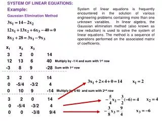
Gaussian Elimination • An algorithm that manipulate an augmented matrix into a “nice” augmented matrix
Row Echelon Form • A matrix is in “Row Echelon Form” (called row echelon matrix) if • All zero rows are at the bottom • The first nonzero entry from the left in each nonzero row is 1 • (that 1 is called a leading 1 of that row) • Each leading 1 is to the right of all leading 1’s in the row above it
Echelon? • Diagonal Formation
Reduced Row Echelon • The leading 1 is the only nonzero element in that column row echelon Reduced row echelon
Theorem 2 • Every matrix can be manipulated into a (reduced) row echelon form by a series of elementary row operations
Using (Reduced) Row Echelon Form No solution
Solution to (c) Variable corresponding to the leading 1’s is called “leading variable” The non-leading variables end up as a parameter in the solution
Gaussian Elimination • If the matrix is all zeroes stop • Find the first column from the left containing a non zero entry (called it A) and move the row having that entry to the top row • Multiply that row by 1/A to create a leading 1 • Subtract multiples of that row from rows below it, making entry in that column to become zero • Repeat the same step from the matrix consists of remaining row
Redundancy Subtract 2 time row 1 from row 2 And Subtract 7 time row 1 from row 3 Subtract 2 time row 2 from row 1 And Subtract 3 time row 2 from row 3
Redundancy redundancy Observe that the last row is the triple of the second row
Back Substitution • Gaussian Elimination brings the matrix into a row echelon form • To create a reduced row echelon form • We need to change step 4 such that it also create zero on the “above” row as well • Usually, that is less efficient • It is better to start from the row echelon form and then use the leading 1 of the bottom-most row to create zero
Another Example Try it
Solution Must be 0
Rank • It is (later) shown that, for any matrix A, it has the same “Reduced row echelon form” • Regardless of the elementary row operation performed • But it s not true for “row echelon form” • Different sequence of operations leads to different row echelon matrix • However, the number of leading 1’s is always the same • Will be proved later • Hence, the number of leading 1’s depends on A • The number of leading 1’s is called rank of A
Theorem 3 • Suppose a system of m equation on n variables has a solution, if the rank of the augmented matrix is r • the set of the solution involve exactly n-r parameters
Homogeneous Equation When b = 0 What is the solution?
Homogeneous Linear System • Xi = 0 is always a solution to the homogeneous system • It is called “trivial” solution • Any solution having nonzero term is called “nontrivial” solution
Existence of Nontrivial Solution to the homogeneous system • If it has non-leading entry in the row echelon form • The solution can be described as a parameter • Then it has nonzero solution!!! • Nontrivial • When will we have non-leading entry? • When we have more variable than equation
Geometrical Point of View • A system of Linear Equation A line in 2D A line in 2D