Download
1 / 42
430 likes | 540 Views
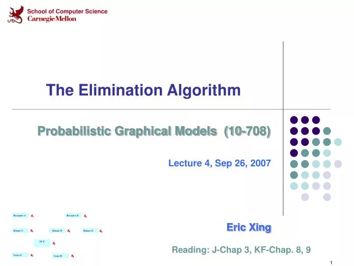
The Elimination Algorithm. Probabilistic Graphical Models (10-708) Lecture 4, Sep 26, 2007 Eric Xing. Reading: J-Chap 3, KF-Chap. 8, 9. Probabilistic Inference. We now have compact representations of probability distributions: Graphical Models

E N D
The Elimination Algorithm Probabilistic Graphical Models (10-708) Lecture 4, Sep 26, 2007 Eric Xing Reading: J-Chap 3, KF-Chap. 8, 9
Probabilistic Inference • We now have compact representations of probability distributions: Graphical Models • A GM G describes a unique probability distribution P • How do we answer queries about P? • We use inference as a name for the process of computing answers to such queries
Query 1: Likelihood • Most of the queries one may ask involve evidence • Evidence e is an assignment of values to a set Evariables in the domain • Without loss of generality E = { Xk+1, …, Xn} • Simplest query: compute probability of evidence • this is often referred to as computing the likelihood of e
Query 2: Conditional Probability • Often we are interested in the conditional probability distribution of a variable given the evidence • this is thea posteriori belief in X, given evidence e • We usually query a subset Y of all domain variables X={Y,Z}and "don't care" about the remaining, Z: • the process of summing out the "don't care" variables z is called marginalization, and the resulting P(y|e) is called a marginalprob.
A A B B C C Applications of a posteriori Belief • Prediction: what is the probability of an outcome given the starting condition • the query node is a descendent of the evidence • Diagnosis: what is the probability of disease/fault given symptoms • the query node an ancestor of the evidence • Learning under partial observation • fill in the unobserved values under an "EM" setting (more later) • The directionality of information flow between variables is not restricted by the directionality of the edges in a GM • probabilistic inference can combine evidence form all parts of the network ? ?
Query 3: Most Probable Assignment • In this query we want to find the most probable joint assignment (MPA) for some variables of interest • Such reasoning is usually performed under some given evidence e, and ignoring (the values of) other variables z: • this is the maximum a posteriori configuration of y.
Applications of MPA • Classification • find most likely label, given the evidence • Explanation • what is the most likely scenario, given the evidence Cautionary note: • The MPA of a variable depends on its "context"---the set of variables been jointly queried • Example: • MPA of X? • MPA of (X, Y) ?
Complexity of Inference Thm: Computing P(X = x|e) in a GM is NP-hard • Hardness does not mean we cannot solve inference • It implies that we cannot find a general procedure that works efficiently for arbitrary GMs • For particular families of GMs, we can have provably efficient procedures
Approaches to inference • Exact inference algorithms • The elimination algorithm • Message-passing algorithm (sum-product, belief propagation) • The junction tree algorithms • Approximate inference techniques • Stochastic simulation / sampling methods • Markov chain Monte Carlo methods • Variational algorithms
E A B C D a naïve summation needs to enumerate over an exponential number of terms Marginalization and Elimination A signal transduction pathway: • Query: P(e) • By chain decomposition, we get What is the likelihood that protein E is active?
E A B C D Elimination on Chains • Rearranging terms ...
E A B C D Elimination on Chains • Now we can perform innermost summation • This summation "eliminates" one variable from our summation argument at a "local cost". X
E A B C D Elimination in Chains • Rearranging and then summing again, we get X X
E A B C D Elimination in Chains • Eliminate nodes one by one all the way to the end, we get X X X X • Complexity: • Each step costs O(|Val(Xi)|*|Val(Xi+1)|) operations: O(kn2) • Compare to naïve evaluation that sums over joint values of n-1 variables O(nk)
E A B C D Undirected Chains • Rearranging terms ...
The Sum-Product Operation • In general, we can view the task at hand as that of computing the value of an expression of the form: where F is a set of factors • We call this task the sum-product inference task.
Outcome of elimination • Let X be some set of variables, let F be a set of factors such that for each f ∈ F, Scope[f ] ⊆ X, let Y ⊂ X be a set of query variables, and let Z = X−Y be the variable to be eliminated • The result of eliminating the variable Zis a factor • This factor does not necessarily correspond to any probability or conditional probability in this network. (example forthcoming)
Dealing with evidence • Conditioning as a Sum-Product Operation • The evidence potential: • Total evidence potential: • Introducing evidence --- restricted factors:
Inference on General GM via Variable Elimination General idea: • Write query in the form • this suggests an "elimination order" of latent variables to be marginalized • Iteratively • Move all irrelevant terms outside of innermost sum • Perform innermost sum, getting a new term • Insert the new term into the product • wrap-up
The elimination algorithm Procedure Elimination ( G, // the GM E, // evidence Z, // Set of variables to be eliminated X, // query variable(s) ) • Initialize (G) • Evidence (E) • Sum-Product-Elimination (F, Z, ≺) • Normalization (F)
Procedure Initialize (G, Z) Let Z1, . . . ,Zk be an ordering of Z such that Zi ≺ Zj iff i < j Initialize F with the full the set of factors Procedure Evidence (E) for eachiÎIE , F =FÈd(Ei, ei) Procedure Sum-Product-Variable-Elimination (F, Z, ≺) for i = 1, . . . , k F ← Sum-Product-Eliminate-Var(F, Zi) f∗ ← Õf∈Ff return f∗ Normalization (f∗) The elimination algorithm
Procedure Initialize (G, Z) Let Z1, . . . ,Zk be an ordering of Z such that Zi ≺ Zj iff i < j Initialize F with the full the set of factors Procedure Evidence (E) for eachiÎIE , F =FÈd(Ei, ei) Procedure Sum-Product-Variable-Elimination (F, Z, ≺) for i = 1, . . . , k F ← Sum-Product-Eliminate-Var(F, Zi) f∗ ← Õf∈Ff return f∗ Normalization (f∗) Procedure Normalization (f∗) P(X|E)=f∗(X)/åxf∗(X) Procedure Sum-Product-Eliminate-Var ( F, // Set of factors Z // Variable to be eliminated ) F ′ ← {f ∈ F : Z ∈ Scope[f]} F ′′ ← F − F ′ y ←Õf∈F ′f t ← åZy return F ′′ ∪ {t} The elimination algorithm
A B D C F E G H A more complex network A food web What is the probability that hawks are leaving given that the grass condition is poor?
A B D C F E G H A B D C F E G Example: Variable Elimination • Query: P(A |h) • Need to eliminate: B,C,D,E,F,G,H • Initial factors: • Choose an elimination order: H,G,F,E,D,C,B • Step 1: • Conditioning (fix the evidence node (i.e., h) to its observed value (i.e., )): • This step is isomorphic to a marginalization step:
A B D C F E G H A B D C F E Example: Variable Elimination • Query: P(B |h) • Need to eliminate: B,C,D,E,F,G • Initial factors: • Step 2: Eliminate G • compute
A B D C F E G H A B D C E Example: Variable Elimination • Query: P(B |h) • Need to eliminate: B,C,D,E,F • Initial factors: • Step 3: Eliminate F • compute
A B D C F E G H A B D C Example: Variable Elimination • Query: P(B |h) • Need to eliminate: B,C,D,E • Initial factors: • Step 4: Eliminate E • compute
A B D C F E G H A B C Example: Variable Elimination • Query: P(B |h) • Need to eliminate: B,C,D • Initial factors: • Step 5: Eliminate D • compute
A B D C F E G H A B Example: Variable Elimination • Query: P(B |h) • Need to eliminate: B,C • Initial factors: • Step 6: Eliminate C • compute
A B D C F E G H Example: Variable Elimination • Query: P(B |h) • Need to eliminate: B • Initial factors: • Step 7: Eliminate B • compute A
A B D C F E G H Example: Variable Elimination • Query: P(B |h) • Need to eliminate: { } • Initial factors: • Step 8: Wrap-up
Complexity of variable elimination • Suppose in one elimination step we compute This requires • multiplications • For each value for x, y1, …, yk, we do k multiplications • additions • For each value of y1, …, yk, we do |Val(X)|additions Complexity is exponentialin number of variables in the intermediate factor
A A B B D D C C A F F E E G G H H A B D C A A A A A B B B B B F E D D D C C C C F E E G Understanding Variable Elimination • A graph elimination algorithm moralization graph elimination
Graph elimination • Begin with the undirected GM or moralized BN • Graph G(V, E) and elimination ordering I • Eliminate next node in the ordering I • Removing the node from the graph • Connecting the remaining neighbors of the nodes • The reconstituted graph G'(V, E') • Retain the edges that were created during the elimination procedure • The graph-theoretic property: the factors resulted during variable elimination are captured by recording the elimination clique
A B A B A A C D C A A B B A E D D C C A F F E E F E G G H H A F E E D C A B H G D C A A A A A B B B B B F E D D D C C C C F E E G Understanding Variable Elimination • A graph elimination algorithm • Intermediate terms correspond to the cliques resulted from elimination moralization graph elimination
A B A B A A C D C A E F E A F E E D C H G Graph elimination and marginalization • Induced dependency during marginalization vs. elimination clique • Summation <-> elimination • Intermediate term <-> elimination clique
Complexity • The overall complexity is determined by the number of the largest elimination clique • What is the largest elimination clique? – a pure graph theoretic question • Tree-widthk: one less than the smallest achievable value of the cardinality of the largest elimination clique, ranging over all possible elimination ordering • “good” elimination orderings lead to small cliques and hence reduce complexity (what will happen if we eliminate "e" first in the above graph?) • Find the best elimination ordering of a graph --- NP-hard Inference is NP-hard • But there often exist "obvious" optimal or near-opt elimination ordering
Examples • Star • Tree
A A B B D D C C A F F E E G G H H A B D C A A A A A B B B B B F E D D D C C C C F E E G Limitation of Procedure Elimination • Limitation
A B A B A A C D C A A B B A E D D C C A F F E E F E G G H H A F E E D C A B H G D C A A A A A B B B B B F E D D D C C C C F E E G From Elimination to Message Passing • Our algorithm so far answers only one query (e.g., on one node), do we need to do a complete elimination for every such query? • Elimination ºmessage passing on a clique tree • Messages can be reused º
A B A B A A C D C A E F E A F E E D C H G From Elimination to Message Passing • Our algorithm so far answers only one query (e.g., on one node), do we need to do a complete elimination for every such query? • Elimination ºmessage passing on a clique tree • Another query ... • Messages mf and mh are reused, others need to be recomputed
Summary • The simple Eliminate algorithm captures the key algorithmic Operation underlying probabilistic inference: --- That of taking a sum over product of potential functions • What can we say about the overall computational complexity of the algorithm? In particular, how can we control the "size" of the summands that appear in the sequence of summation operation. • The computational complexity of the Eliminate algorithm can be reduced to purely graph-theoretic considerations. • This graph interpretation will also provide hints about how to design improved inference algorithm that overcome the limitation of Eliminate.