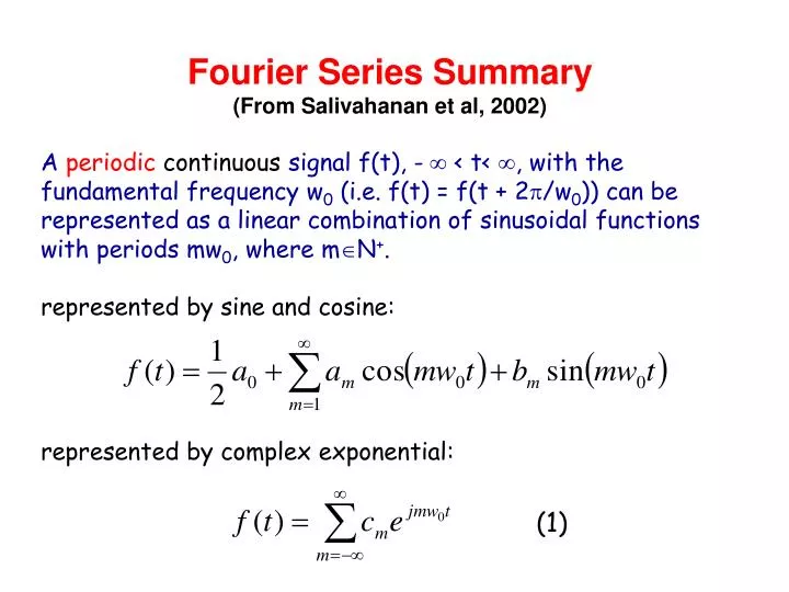
Fourier Series Summary (From Salivahanan et al, 2002)

1. Fourier Series Summary (From Salivahanan et al, 2002) A periodiccontinuous signal f(t), - < t< , with the fundamental frequency w0 (i.e. f(t) = f(t + 2/w0)) can be represented as a linear combination of sinusoidal functions with periods mw0, where mN+. represented by sine and cosine: represented by complex exponential: (1)

2. am and bm can be resolved as represented by complex exponential: (2) cm and c-m are complex conjugate pairs

3. The integral can also be performed within [0, 2/w0] More concise relation between {am, bm} and cm: In (1) and (2), f(t) and cm(- < t< , mZ) form a transform pair, where (2) is referred to as a forward transform, and (1) is an inverse transform. • Fourier series specifies Fourier transform in situation of periodic signals.

4. Frequency domain: we say that the periodic signal f(t) is transformed to the frequency domain specified by mw0 (mZ) by Fourier series. cm is the frequency component of f(t) with respect to the frequency mw0. • The frequency domain (or spectrum) or a periodic continuous signal is discrete. • In contrast, the domain which the signal is defined is referred to as the “time domain” or “space domain.” The frequency components cm is a complex number. Hence, the transform domain can be divided into two parts: magnitude and phase.

5. Example: f(t) 5 …… 0 2 4 6 8 …… w0t (only when m > 0)

6. |Cm| 5/2 5/2 5/4 w 0 w0 2w0 3w0 …… • when m=0, c-m is cm’s complex conjugate, so • magnitude in the transform domain (in this case, the magnitude is an even function that is symmetric to the y-axis)

7. Cm /2 … 3w02w0w0 w 0 w0 2w0 3w0 …… /2 • phase in the transform domain: (it is an odd function) • The frequency domain of a Fourier transform contains both the magnitude and phase spectra. • High frequency (w=mw0 is large): corresponds to the signal components that highly vary with time. • Low frequency (w=mw0 is small) corresponds to the signal components that slowly vary with time.

8. Parserval’s Theorem for Fourier series Remember that

9. We have In general, Parserval’s theorem means “energy preservation.” power of a periodic signal: power in the frequency domain:

10. Continuous Fourier Transform Fourier series transforms a periodic continuous signal into the frequency domain. What will happen when the continuous signal is not periodic? Consider the period of a signal with the fundamental frequency being w0: (note that T specifies the fundamental period instead of the time step defined before) A non-periodic signal can be conceptually thought of as a periodic signal whose fundamental period T is infinite long, T . In this case, the fundamental period w0 0.

11. Remember that the spectrum (in the frequency domain) of a periodic continuous signal is discrete, specified by mw0 (mZ). The interval between adjacent frequencies is w0. When w0 0, we can image that the frequency becomes continuous: (where the interval w0becomes dw) The summation in the inverse transform becomes integral. Thus,

12. Continuous Fourier Transform: • The forward transform: • The inverse transform: The continuous Fourier transform has very similar forward and inverse forms. The only difference is that the forward uses –j and the inverse uses j in the complex exponential basis. This suggests that the roles of time and frequency can be exchanged, and some properties are symmetric to each other. Both time and frequency domains in continuous Fourier transform are continuous. The frequency waveform is also referred to as the ‘spectrum’.

13. Many variations of forms of continuous F. T. From Kuhn 2005

15. From Kuhn 2005

17. What is the continuous Fourier transform of a periodic signal?

19. F(jw) 5/2 5/2 5/4 w 0 w0 2w0 3w0 …… Dirac’s delta functionis also called unit impulse function. The unit impulse function (t) can be multiplied by a real number r (or a complex number c), say r(t) (or c(t)), to represent the delta function of different magnitudes (or magnitudes/angles). The continuous Fourier transform of a periodic signal is a impulse train. Relationship to the discrete Fourier series: the magnitudes of the impulse functions are proportional to those computed from the discrete Fourier series.

20. Periodic signal examples

21. Discrete Time Fourier Transform (DTFT) From Fourier Series Time domain is periodic  frequency domain is discrete Remember that the continuous Fourier transform has similar forms of forward and inverse transforms. Question: When time domain is discrete, what happens in the frequency domain?  The frequency domain is periodic Discrete time Fourier transform: time domain: a discrete-time signal …, x[-2T], x[-T], x[0], x[T], x[2T], … (T is the time step)

22. Energy signal and power signal

23. Forward transform of DTFT: Property: Forward DTFT is periodic with the period ws = 2/T. pf: Let r be any integers, then Since X(ejwt) is periodic, according the Fourier series principle, it can be expressed in the time domain as a linear combination of complex exponentials, as the form shown in the forward DTFT. The coefficients of the linear combination can then be computed by finding the integral over a period: Inverse transform of DTFT:

24. If we skip the time step T (or simply T=1): forward DTFT: inverse DTFT: In this case,DTFT is periodic with the period being 2. In digital signal processing, discrete-time signals are of the main interest, and DTFT is a main tool for analyzing such a signal. Since the frequency spectrum repeats periodically with the period 2, we usually consider only a finite-duration [,] (or [0, 2]). High frequency region: The frequency nearing  or . Low frequency region: The frequency nearing 0.

25. Aliasing Effect (c.f. Shenoi, 2006) Find the relationship between the continuous Fourier transform Xa(j) of the continuous function xa(t) and the DTFT X(ejwT). Notation of continuous Fourier transform: forward inverse Assume that the discrete-time signal x(nT) is uniformly sampled from the analog signal xa(t) with the time step T. Apply the inverse Fourier transform, we have

26. Let’s express this equation, which involves integration from = to =, as the sum of integrals over successive intervals each equal to one period 2/T = ws. However, each term in this summation can be reduced to an integral over the range /T to /T by changing a variable from  to +2r/T: Note that ej2rn = 1 for all integers r and n. By changing the order of summation and integration, we have

27. Without loss of generality, we change the frequency variable  to w, Comparing the above equation with that of the inverse DTFT, We get the desired relationship (between DTFT and continuous Fourier transform):

28. This shows that DTFT of the sequence x(nT) generated by sampling the continuous signal xa(t) with a sampling period T is obtained by a periodic duplication of the continuous Fourier transform Xa(jw) of xa(t) with a period 2/T = ws and scaled by T. Because of the overlapping effect, more commonly known as “aliasing,” there is no way of retrieving Xa(jw) from X(ejwT); in other words, we have lost the information contained in the analog function xa(t) when we sample it. See figure explanation: (Note that when xa(t) is a real-number signal, then the magnitude of its Fourier transform is an even function, i.e., is symmetric to the y-axis).

30. Sampling Theorem (c.f. Shenoi, 2006) When can we reconstruct the continuous signal from its uniform sampling? iff • the continuous signal xa(t) is band limited – that is, if it is a function such that its Fourier transform Xa(jw) = 0 for |w|>2wb, where wb is a frequency bound. • the sampling period T is chosen such that ws > 2 wb (where wsT=2). • That is, to avoid the situation of aliasing, the sampling frequency shall be larger than twice of the highest frequency of the continuous signal. • Nyquist sampling theorem: fb (wb/2) is called the Nyquist frequency, and 2fb is called the Nyquist rate. See figures for explanation.

31. Sampled signal Continuous signal The magnitude spectrum of the continuous signal The spectrum of the sampled signal

32. Particular discrete-time signal examples • Unit pulse (or unit sample) function (or discrete-time impulse; impulse)

33. An arbitrary sequence x[n], nZ can be represented as a sum of scaled, delayed impulses.

34. Unit step sequence

35. Some DTFT Transform Pairs

36. DTFT Transform Pairs (continue)

37. DTFT Transform Pairs (continue)

38. DTFT Theorems • Linearity x1[n]  X1(ejw), x2[n]  X2(ejw) implies that a1x1[n] + a2x2[n]  a1X1(ejw) + a2X2(ejw) • Time shifting x[n]  X(ejw) implies that

39. DTFT Theorems (continue) • Frequency shifting x[n]  X(ejw) implies that • Time reversal x[n]  X(ejw) If the sequence is time reversed, then x[n]  X(ejw)

40. DTFT Theorems (continue) • Differentiation in frequency x[n]  X(ejw) implies that • Parseval’s theorem x[n]  X(ejw) implies that

41. Example • Suppose we wish to find the Fourier transform of x[n] = anu[n-5].

42. Representation of Sequences by Discrete-time Fourier Transforms(DTFT)(cf. Oppenheim et al. 1999) • Fourier Representation: representing a signal by complex exponentials. • A signal x[n] is represented as the Fourier integral of the complex exponentials in the range of frequencies [,]. • The weight X(ejw) of the frequency applied in the integral can be determined by the input signal x[n], and X(ejw) reveals how much of each frequency is required to synthesize x[n]. Inverse Fourier transform Fourier transform (or forward Fourier transform)

43. Representation of sequences by DTFT (continue) • The phase X(ejw) is not uniquely specified since any integer multiple of 2 may be added to X(ejw) at any value of w without affecting the result. • Denote ARG[X(ejw)] to be the phase value in [,]. • Since the frequency response of a LTI system is the Fourier transform of the impulse response, the impulse response can be obtained from the frequency response by applying the inverse Fourier transform integral:

44. Existence of discrete-time Fourier transform pairs • Whey they are transform pairs? Consider the integral

45. Conditions for the existence of discrete-time Fourier transform pairs • Conditions for the existence of Fourier transform pairs of a signal: • Absolutely summable • Mean-square convergence: In other words, the error |X(ejw)  XM(ejw) | may not approach for each w, but the total “energy” in the error does.

46. Conditions for the Existence of DTFT transform Pairs (continue) • Still some other cases that are neither absolutely summable nor mean-square convergence, the Fourier transform still exist: • Eg., Fourier transform of a constant, x[n] = 1 for all n, is an impulse train: • The impulse of the continuous case is a “infinite heigh, zero width, and unit area” function. If some properties are defined for the impulse function, then the Fourier transform pair involving impulses can be well defined too.

47. Symmetry Property of the Fourier Transform • Conjugate-symmetric sequence: xe[n] = xe*[n] • If a real sequence is conjugate symmetric, then it is called an even sequence satisfying xe[n] = xe[n]. • Conjugate-asymmetric sequence: xo[n] = xo*[n] • If a real sequence is conjugate antisymmetric, then it is called an odd sequence satisfying x0[n] =  x0[n]. • Any sequence can be represented as a sum of a conjugate-symmetric and asymmetric sequences, x[n] =xe[n] + xo[n], where xe[n] = (1/2)(x[n]+ x*[n]) and xo[n] = (1/2)(x[n]  x*[n]).

48. Symmetry Property of the Fourier Transform (continue) • Similarly, a Fourier transform can be decomposed into a sum of conjugate-symmetric and anti-symmetric parts: X(ejw) = Xe(ejw) + Xo(ejw) , where Xe(ejw) = (1/2)[X(ejw) + X*(ejw)] and Xo(ejw) = (1/2)[X(ejw)  X*(ejw)]

49. Symmetry Property of the Fourier Transform (continue) • Fourier Transform Pairs (if x[n]  X(ejw)) • x*[n]  X*(e jw) • x*[n]  X*(ejw) • Re{x[n]}  Xe(ejw) (conjugate-symmetry part ofX(ejw)) • jIm{x[n]}  Xo(ejw) (conjugate anti-symmetry part ofX(ejw)) • xe[n] (conjugate-symmetry part ofx[n])  XR(ejw) = Re{X(ejw)} • xo[n] (conjugate anti-symmetry part ofx[n])  jXI(ejw) = jIm{X(ejw)}

50. Symmetry Property of the Fourier Transform (continue) • Fourier Transform Pairs (if x[n]  X(ejw)) • Any realxe[n]  X(ejw) = X*(ejw) (Fourier transform is conjugate symmetric) • Any realxe[n]  XR(ejw) = XR(ejw) (real part is even) • Any realxe[n]  XI(ejw) = XI(ejw) (imaginary part is odd) • Any realxe[n]  |XR(ejw)| = |XR(ejw)| (magnitude is even) • Any realxe[n]  XR(ejw)= XR(ejw) (phase is odd) • xo[n] (even part of realx[n])  XR(ejw) • xo[n] (odd part of realx[n])  jXI(ejw)