Download
1 / 30
400 likes | 625 Views
CEE162/262c Lecture 14: Continuous Stochasticity. figure(2) plot(t,N(:,1:100), 'k.-' ); xlabel( 't' ); ylabel( 'N(t)' ); figure(3) plot(t,exp(-lambda*t), 'r-' , ... t,lambda*t.*exp(-lambda*t), 'g-' , ... t,(lambda*t).^2/2.*exp(-lambda*t), 'b-' , ... t,num(1:3,:), 'k.' );

E N D
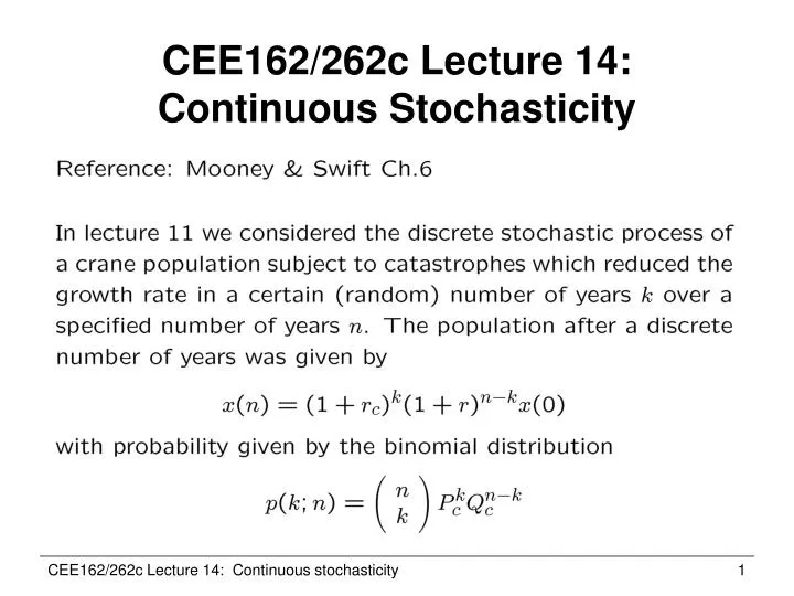
CEE162/262c Lecture 14: Continuous Stochasticity CEE162/262c Lecture 14: Continuous stochasticity
figure(2) plot(t,N(:,1:100),'k.-'); xlabel('t'); ylabel('N(t)'); figure(3) plot(t,exp(-lambda*t),'r-',... t,lambda*t.*exp(-lambda*t),'g-',... t,(lambda*t).^2/2.*exp(-lambda*t),'b-',... t,num(1:3,:),'k.'); legend('n=0','n=1','n=2',1); xlabel('t'); ylabel('P_n(t)'); figure(4) plot([0:Nmax],num(:,nsteps/4),'r-',... [0:Nmax],num(:,nsteps/2),'g-',... [0:Nmax],num(:,3*nsteps/4),'b-',... [0:Nmax],num(:,nsteps),'m-'); legend('T/4','T/2','3T/4','T'); xlabel('N'); ylabel('p(N,t)'); figure(5); Nbar = mean(N,2); plot(t,Nbar,'k-'); xlabel('t'); ylabel('mean(N(t))'); % File: unserved.m lambda = .1; % Arrival rate T = 80; nsteps = 400; dt = T/nsteps; numtrials = 10000; N = zeros(nsteps,numtrials); grow = rand(nsteps,numtrials)<lambda*dt; N = cumsum(grow); Nmax = max(max(N)); [num,x] = hist(N',[0:Nmax]); num = num/numtrials; t = [dt:dt:dt*nsteps]; [T,X] = meshgrid(t,x); figure(1) mesh(T(:,1:10:end),X(:,1:10:end),num(:,1:10:end)); xlabel('t'); ylabel('N'); zlabel('p(N,t)'); CEE162/262c Lecture 14: Continuous stochasticity
Figure 1 CEE162/262c Lecture 14: Continuous stochasticity
Fig. 3 Fig. 2 Fig. 5 Fig. 4 CEE162/262c Lecture 14: Continuous stochasticity
Nmax = max(max(N)); [num,x] = hist(N',[0:Nmax]); num = num/numtrials; t = [dt:dt:dt*nsteps]; figure(1) plot(t,N(:,1:10),'k-'); xlabel('t'); ylabel('N(t)'); figure(2) onest = ones(size(t)); plot(t,(1-rho)*onest,'r-',... t,rho*(1-rho)*onest,'g-',... t,rho^2*(1-rho)*onest,'b-',... t,num(1:3,:),'k.'); legend('n=0','n=1','n=2',1); xlabel('t'); ylabel('P_n(t)'); % File: singleserverqueue.m Ns=2; % Steady-state # of customers in line rho = Ns/(1+Ns);% Traffic intensity lambda = .1; % Arrival rate mu = lambda/rho;% Service rate T = 1000; nsteps = 4000; dt = T/nsteps; numtrials = 4000; N = zeros(nsteps,numtrials); for trial=1:numtrials fprintf('Trial %d of %d\n',trial,numtrials); for n=2:nsteps P=rand<(lambda*dt); Q=rand<(mu*dt); if(P==1 & Q==1) r=rand; P=P*(r<0.5); Q=Q*(r>=0.5); end N(n,trial)=N(n-1,trial)+P-(Q & N(n-1,trial)>0); end end CEE162/262c Lecture 14: Continuous stochasticity
% Compute the power series to get the second moment of N % First moment is known analytically E1 = rho/(1-rho); % Second moment is compute numerically n = [0:100]; E2 = sum(n.^2.*rho.^n*(1-rho)); sig = sqrt(E2-E1^2); figure(3); Nbar = mean(N,2)'; Nstd = std(N')'; Nmean = rho/(1-rho); plot(t,Nbar,'k-',... t,Nstd,'r-',... [0 max(t)],[E1 E1],'k--',... [0 max(t)],[sig sig],'r--'); legend('Mean','Std',4);xlabel('t');ylabel('mean(N(t))'); CEE162/262c Lecture 14: Continuous stochasticity
Fig. 1 Fig. 3 Fig. 2 CEE162/262c Lecture 14: Continuous stochasticity