Naïve Bayes

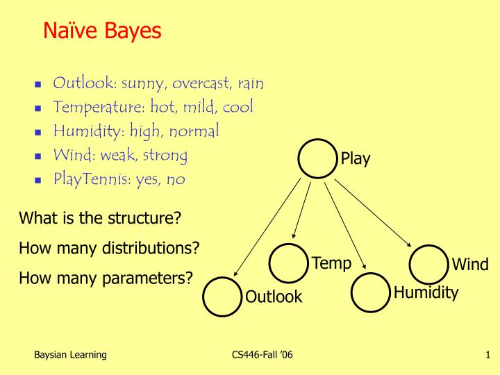
1. Outlook Temp Humidity Wind Play Naïve Bayes • Outlook: sunny, overcast, rain • Temperature: hot, mild, cool • Humidity: high, normal • Wind: weak, strong • PlayTennis: yes, no What is the structure? How many distributions? How many parameters? CS446-Fall ’06

2. Strong Assumptions • Each category of interest to be inferredCavity vs. No Cavity OR Play vs. Can’t Playis modeled linearly • Linear = independent = Markov = no interactions = easy • Log probability of category is a hyperplane • Generative model • Calculate the probability of each assignment • Choose the higher (highest) one • What is the decision surface?i.e., what space of discriminative models are we committing to? • What about BNs generally (not just NB)? CS446-Fall ’06

3. Are Our NB Assumptions Valid? • Are Temperature and Humidity independent given that I cannot play tennis today? • Definitely not! • Note the difference with the cavity naïve Bayes network • In cavity NB network • We believe our conditional independence assumptions • Incidentally it turns out to fit naïve Bayes • In the tennis NB network • We do NOT believe our C.I. assumptions • We make them anyway to simplify modeling CS446-Fall ’06

4. We often intentionally simplify the model • What are we sacrificing? • modeling fidelity, • interactions, • accuracy… • How does this consciously incorrect modeling manifest itself? • increased “apparent” randomness in the world; • higher variances • What do we gain? • a less expressive hypothesis space, • faster learning / convergence • Do it carefully! CS446-Fall ’06

5. Often such simplifications still result in good performance • Why? • Many analyses have been offered – some quite technical • Probably a number of reasons • Tends to leave out low order detailsOften “linear” is the dominant or most important influence • Simplified model  fewer parametersSame size data set  information & confidence is concentrated in those parameters that model the dominant effects • We get to choose the “evidence” features; barometric pressure; yesterday’s weather, how long since I played tennis… Intuitively (or by trial and error), we avoid features with important strong interactions CS446-Fall ’06

6. Back to General Bayes / Parameterized ModelsLatent Variables, Missing Values, and the EM Algorithm • What if we cannot observe some features? • These are latent variables, making (even) the training data incomplete(Also works for non-systematically missing values) • Some of the most interesting variables are latent (unobservable):applicant’s honesty, intent to pay back a loan, future auto reliability and repair costs, existence of heart muscle decay… • Not necessarily classification labels; want a generative model that respects the existence of latent (unobservable) features • We know the relations among variables (say, the Bayes net structure) • We observe values for some variables • What can we do? CS446-Fall ’06

7. EM (Expectation Maximization) Algorithm(magical version) • We want the parameter values (CPT entries) that make the observed data most likely • We need parameter values for latent random variables • EM: • We make our best guesses about the missing data • Then we infer missing parameters from these guesses • These parameter values are probably wrong so we repeat the process • Stop at convergence • Magical part: • The process converges… • But to a local optimum • It often does quite well • Convergence can be slow • How? Why? Where does the information come from? • Short demystifying answer: • The known / assumed structure couples observed features to the parameters that describe the latent ones • If the latent variables had no influence they would NOT be included in the parameterized model • Their presence indicates some informational exposure of their parameters to the observed data CS446-Fall ’06

8. EM – Expectation / Maximization • EM is a class of algorithms that is used to estimate a probability distribution in the presence of missing values. • Using it, requires an assumption on the underlying probability distribution. • The algorithm can be very sensitive to this assumption and to the starting point (that is, the initial guess of parameters). • It is a hill-climbing algorithm and converges to a local maximum of the likelihood function. CS446-Fall ’06

9. The Likelihood Function • Set of training data D • A parametric family of models w/ parameters  • We want  that maximizes Pr( | D) • Bayes: Pr( | D) = Pr(D | ) * Pr() / Pr(D) • Pr(D | ) when viewed as a function of  is called the likelihood function: L(;D) = Pr(D | ) sometimes L(,D) L(D | ) • The likelihood function is NOT a probability distribution over  and its integral / sum need not be 1.0 • The M.L. (maximum likelihood) , is the one that maximizes the likelihood function (without regard for a prior on ) CS446-Fall ’06

10. L  M.L.  The Likelihood Function • We would like the maximum likelihood  even though D is incomplete • The likelihood function may not be smooth or unimodal • Analytic solutions are often difficult or impossible CS446-Fall ’06

11. Intuitive Example: K-Means Clustering • Clustering = unsupervised learning • (More on clustering later in the semester) • Suppose we know that k processes generate data stochastically • Each process generates normally distributed data although the normal distributions are different • Only the means differ;variances are the same and k=2. • We do not know which data point was generated by which process • Which process generated it is a latent variable of each datum CS446-Fall ’06

12. K-Means Problem We observe the green data points Independent samples from 2 Normal distributions Different means but a common standard deviation. Estimate the means i, i=1,…k=2and the standard deviation  from the data CS446-Fall ’06

13. Maximum Likelihood, Full Observability If only we knew which process produced which data point, finding the most likely parameters would be easy. We get many data points, D = {x1,…,xm} Maximizing the log-likelihood is equivalent to minimizing: Calculate the derivative with respect to , we get that the minimal point, that is, the most likely mean is CS446-Fall ’06

14. A Mixture of Distributions We do not know how each data point xi was generated We do know the general parameterized form of the probability that observed data point xi was generated by distribution j: j: CS446-Fall ’06

15. A Mixture of Distributions Let X={x1,…xm} be the observed data (m independent samples) For each data point xi, define k binary hidden variables, zi1,zi2,…,zik s.t zij =1 iff xi is sampled from the j-th distribution. Let Y be the complete data. E[V] is the expectation of V; Recall E is a linear operator CS446-Fall ’06

16. Example: k-means Algorithm Expectation: Computing the likelihood given the observed data D = {x1,…,xm} and the hypothesis h (w/o the constant coefficient) CS446-Fall ’06

17. Example: k-means Algorithm Maximization: Maximizing with respect to we get that: Which yields: CS446-Fall ’06

18. k-means Algorithm Given a set D = {x1,…,xm} of data points, guess initial parameters Compute (for all i,j) Compute M.L. parameters: repeat to convergence Expectation: assignment of hidden values Maximization: updating parameters Notice that this algorithm will find the best k means in the sense of minimizing the sum of square distance. CS446-Fall ’06

19. The EM Algorithm • Algorithm: • Guess initial values for the hypothesis h= • Expectation: • Calculate expected values for Z’s and Y • Calculate Q(h’|h) = E(Log P(Y|h’) | h, X) • using the current hypothesis h and the observed data X. • Maximization: • Replace the current hypothesis h by h’, that maximizes • the Q function • Choose set h’ such that Q(h’|h) is maximal • Set h = h’ • Repeat: Estimate the Expectation again. CS446-Fall ’06

20. L  M.L.  EM • Performs Hill Climbing • A locally optimal fit is found • Convergence to local optimal may be slow • Fast changes followed by slow ones followed by fast ones… CS446-Fall ’06

21. Three Coin Example • We observe a series of coin tosses generated in the following way: • A person has three coins. • Coin 0: probability of Head is  • Coin 1: probability of Head p • Coin 2: probability of Head q • Consider the following coin-tossing scenario: CS446-Fall ’06

22. Three Coin Problem Toss coin 0. If Head – toss coin 1 four times if Tails – toss coin 2 four times Generating the sequenceHHHHT, THTHT, HHHHT, HHTTH, … produced by Coin 0 , Coin1 and Coin2 Erase the result of flipping coin 0 (the red flips) Observing the sequence HHHT, HTHT, HHHT, HTTH, … produced by Coin 1 and/or Coin 2 Estimate most likely values for p, q and  There is no known analytical solution to computing parameters that maximize the likelihood of the data CS446-Fall ’06

23. Recall • If we knew which of the data points (HHHT), (HTHT), (HTTH) came from Coin1 and which from Coin2, there is no difficulty. • Recall that the “simple” estimation is the ML estimation: • Assume that you toss a (p,1-p) coin m times and get k Heads m-k Tails. log(P(D|p) = log [ pk (1-p)m-k ]= k log p + (m-k) log (1-p) • To maximize, set the derivative w.r.t. p equal to 0: d log P(D|p)/dp = k/p – (m-k)/(1-p) = 0 • Solving this for p, gives: p=k/m CS446-Fall ’06

24. EM Algorithm (Coins) - I • If we knew the parameters we could estimate which coin generated which sequence • Then, we will use the estimation for the tossed Coin, to compute updated most likely parameters and so on... • What is the probability that the ith data point came from Coin1 ? CS446-Fall ’06

25. EM Algorithm (Coins) - II • At this point we would like to compute the likelihood of the data, and find the parameters that maximize it. • We will maximize the log likelihood of the data (n data points): LL = in logP(Di |p,q,) • But, one of the variables – the coin’s name - is hidden. • Which value do we plug in for it in order to compute the likelihood of the data? • We marginalize over it. Or, equivalently, we think of the likelihood log(Di|p,q,) as a random variable that depends on the value of the coin in the ith toss. Therefore, instead of maximizing the LL we will maximize the expectation of this random variable (over the coin’s name). CS446-Fall ’06

26. EM Algorithm (Coins) - III • We maximize the expectation of this random variable (over the coin name). • Due to the linearity of the expectation and the random variable: CS446-Fall ’06

27. EM Algorithm (Coins) - IV • Explicitly, we get: CS446-Fall ’06

28. EM Algorithm (Coins) - V • Finally, to find the most likely parameters, we maximize the derivatives with respect to : CS446-Fall ’06

29. The EM Algorithm • Unsupervised learning: estimation of a probability distribution • There are unobserved variables • Examples: Context variables; Mixture of distribution • The probability distribution is known; the problem is to estimate its parameters • In the case of a mixture: the participating distributions are known, we need to estimate: • - Parameters of the distributions • - The mixture policy • Our previous example: Mixture of Bernuli distributions CS446-Fall ’06

30. The EM Algorithm • Let X={x1,…xm} be the observed data (m independent samples) • Let z={z1,…,zm} be the corresponding unobserved data • Let Y be the complete data. • Maximum Likelihood Approach: Maximize P(Y|h’) (Log(P(Y|h’) ) • Since Y itself is a random variable, we will seek to • Maximize E(Log P(Y|h’) ) • Where the expectation is over the values of Y • h: the current hypothesis for the parameters of the target distribution • We can then evaluate: Q(h’|h) = E(Log P(Y|h’) | h, X) CS446-Fall ’06

31. The EM Algorithm • Algorithm: Guess initial values for the hypothesis h • Estimation: Calculate Q(h’|h) = E(Log P(Y|h’) | h, X) • using the current hypothesis h and the observed data X. • This gives an expression for the most likely distribution • over Y (I.e., estimate the probability distribution over Y) • as a function of the (new) parameters h’ • Maximization: Replace the current hypothesis h by h’, that maximizes the Q function (the likelihood function) • set h = h’, such that Q(h’|h) is maximal • Repeat: Estimate the Expectation again. • EM will converge to a local maximum of the likelihood function P(Y|h’) • Can be used by starting a few times, from different starting points. CS446-Fall ’06

32. Summary: EM • EM is a general procedure for learning in the presence of • unobservable variables. • We have shown how to use it in order to estimate the most likely density function for a mixture of probability distributions. • EM is an iterative algorithm that can be shown to converge to • a local maximum of the likelihood function. • It depends on assuming a family of probability distributions. • It has been shown to be quite useful in practice, when the assumption made on the probability distribution are correct, but can fail otherwise. • As an example, we have derived an important clustering algorithm, the k-means algorithm, as a limit of EM. CS446-Fall ’06