Download
1 / 48
480 likes | 720 Views
Ammonia Toxicity Model AMMTOX. Training Session Held 5 Dec 2005 Hosted by EPA Region VIII Presented by Jim Saunders, Colorado WQCD. Purpose of Training Session. Explain rationale for model Identify data needs and sources, including options for use of site-specific data

E N D
Ammonia Toxicity ModelAMMTOX Training Session Held 5 Dec 2005 Hosted by EPA Region VIII Presented by Jim Saunders, Colorado WQCD
Purpose of Training Session • Explain rationale for model • Identify data needs and sources, including options for use of site-specific data • Demonstrate operation of model • Work with test data sets
Assumptions and Disclaimers • Familiarity with Excel is assumed • VB programming is NOT covered • Future tech support is not my job • Merits of National Criteria are not open for discussion • Ideas and suggestions presented in this session may not conform to policies of state or federal permitting agencies
Section 1: Concepts and Construction Central Question: Where is there greatest risk of exceeding stream standard? Depends on pollutant behavior and control of toxicity
How do you handle a problem like Ammonia? • Calculating permit limits becomes difficult when controlling conditions are displaced downstream • Good news: solution likely to benefit discharger
Pattern of Toxicity, Simple Scenario • Initial • pH: 6.6 • Temp: 16.3 • Final • pH: 8.0 • Temp: 10 • Rebound • pH: 0.2/mi • Temp: 0.7/mi
Pattern of Toxicity, Complex Scenario • Simple Scenario pH, temperature • Initial ammonia = 5.5 • Loss = 3/d • V= 2 fps
Required Tasks • Define d/s trajectory of stream standard • Define d/s trajectory of ammonia concentration • Determine maximum effluent concentration such that instream ammonia will not exceed standard at any point downstream
Trajectory of Standard • Effect of effluent on stream chemistry generally elevates standard • Effect is transitory • Initial value of standard declines downstream because underlying controls (pH and temperature) trend separately toward “equilibrium” values • Greatest risk of exceedance may occur anywhere between outfall and equilibrium conditions
What is equilibrium? • Stable pH and temperature characteristic of this mixture of effluent and stream water • May differ from upstream conditions, especially if effluent flow is large • Equilibrium is dynamic with substantial diel and seasonal variation in pH and temperature • This variability must be captured in standard
Trajectories for pH and Temperature • Initial mixed conditions defined from flow-weighted mean pH and temperature • Effect of effluent on stream pH and temperature is transitory • Initial mixed pH and temperature trend separately toward “equilibrium” values • If the equilibrium value and the rate of change are known, pH or temperature can be predicted at any point downstream of the outfall
Setpoint: Equilibrium with Regulatory Twist • pH and temperature associated with greatest risk of exceeding ammonia standard for equilibrium conditions • Worst case in each month, subject to once-in-three-year exceedance • Terminus for pH and temperature trajectories, not a fixed location
Why Obtaining Setpoint is Difficult • Sole task of Recur model • Field grab samples form framework • Apply characteristics of temporal variation to construct set of hourly values spanning entire period of record • Calculate standards hourly and determine acute (1-h) and chronic (30-d) values consistent with once-in-three-year exceedance threshold • Find associated pH (acute and chronic) and temperature (chronic)
Application for Setpoint • Hidden hand – guides pH and temperature toward target with regulatory meaning • Essential for producing d/s trajectory of ammonia standard, separately for acute and chronic
Back up a step....Incorporation of temporal variation • pH and temperature in stream exhibit temporal variation of diel and seasonal scales...thus applies to standard, too • Predictable diel pattern • Based on sine curve • Given amplitude and time of max, one grab value can define complete 24-h pattern • Model contains defaults, or user can supply
Diel Patterns of Variation • Pattern of each is predictable (sine curve) • Asynchronous pH and temperature patterns
Adjusting Grab Sample Data • Translate grab sample to daily average or maximum using amplitude and time of maximum
Implications for Toxicity • Time of day matters • Not a sine function • Average toxicity is not same as toxicity based on average pH and temperature
Empirical Seasonal Pattern • Driven by pattern observed in recent historical record • Temperature shows strong seasonal variation in mean; tracking air temperature • pH shows strong seasonal variation in amplitude; result of biological activity
Seasonal Variation: Temperature • Strong pattern • Monthly time step • Importance of physical processes
Seasonal Variation: pH • Seasonal change in maxima, but not in minima • Amplitude varies across sites in same region • Importance of biological processes
Next Task: Ammonia Trajectory • Initial concentration determined by mass balance calculations • Change in concentration d/s affected strongly by biological processes (i.e., non-conservative behavior) • Dominant process: nitrification • Others: uptake (-), ammonification (+) • Model represents a net loss rate
Why Non-conservative Matters • Nitrification reduces ammonia • First order kinetics • Any loss increases limits
K3 Temperature Dependence • Nominal rate applies at 20oC • Ambient rate sensitive to temperature (8%/oC)
Revisit Scenario with New K3 • Interaction of loss rate and d/s trajectory of standard • Importance of site-specific data
Next Task: Linking Limits to Standards • AMMTOX sets monthly limits by manual iteration (i.e., trial and error) • Aiming for maximum effluent concentration such that instream ammonia will not exceed standard at any point downstream
Organization of AMMTOX • Recurrence model • Defines setpoint conditions, integral to mapping downstream trajectory of toxicity • Reach Model • Predicts downstream pattern of stream standard based on expected spatial patterns in pH and temperature • Predicts downstream changes in total ammonia based on first order kinetics • Employs graphical approach for setting permit limits
Section 2: Data Needs and Sources • Setpoint Determination • Grab samples from equilibrium stream conditions; 3-5 yrs, weekly-monthly • Diel patterns of variation for pH and temperature (amplitude, time of max) • Default (3 levels for pH) • User supplied (confirm or replace default) • Ecological Conditions • Implied by classification (warm vs. cold) • Local knowledge of fish community
Sampling Site Selection • Ideal site: far enough downstream for rebound to be complete, yet not influenced by tributaries, etc. • Practical site • Upstream OK if too many confounding influences downstream • Small effluent: upstream or 2-4 mi downstream • Large effluent: trajectory based on interim sites
Site-Specific Characterization of Diel Patterns of Variation • Summer (July-August best) • Low flow • Data logger: 15-min intervals; get amplitude and time of max • Grab: sunrise for minima, mid- to late afternoon for maxima; get amplitude • With either approach, a few sunny days will determine usefulness of defaults
Define Ecological Setting for Reach Model • Are salmonids present? • Default assumption might be yes for Cold water classification • Affects pH component (applies to acute and chronic standards) • Are Early Life Stages (ELS) present? • Must specify for each month • Applies to all species in fish community • Affects temperature component (does not apply to acute)
Acute Values (CMC) • 1-h average • Nonlinear function of pH • Not a function of temperature • Linear function of FAV • Salmonids present: 11.23 • Salmonids absent: 16.8
Temperature Dependence and ELS • T<7oC; max effect of ELS • 7<T<14.5oC; diminishing effect • T>14.5oC; no effect of ELS
Chronic Values (CCC) • 30-d average • Nonlinear function of pH • Linear function of FAV • Nonlinear function at higher temperature • Invertebrate slope: 10-0.028*(T-25); T>7oC • Linear function at lower temperature • ELS absent; invertebrate GMCV (1.45) applies at T<7 • ELS present; fish GMCV (2.85) applies at T<14.5
Reach Model Inputs • Flows • Water Quality • Basis for trajectories • Rebound • Setpoint • K3 • Travel time • Characteristics of standards • Consistency with Recur Model (not linked)
Hydrologic Conditions • Upstream: Regulatory low flow (e.g., DFLOW) • Effluent: Design capacity • Tributaries and diversions: preserve low flow regime; reconstructions and DFLOW by difference • Seepage: Residual between gages; includes alluvial discharge, direct surface runoff and small, ungaged tributaries
Input Water Quality • Avoid worst of worst scenarios • Upstream: average or median • Effluent (pH, temperature): average or median • Seepage: average or median • Diversions: no direct effect on WQ
Rebound Rates • Default rates used in AMMTOX • pH: 0.2 units per mile • Temperature: 0.7 oC per mile • Site-specific rates are very rare • Produces gradual, linear shift toward setpoint conditions
Spatial Patterns of Variation • Addition of effluent changes temperature and depresses pH in stream • Shift is transitory, but can be dramatic
Ammonia Loss Rate • Measured for many CO streams • Wide range of values; generous default • Study design considerations • Paired samples d/s of mixing zone • Travel time critical; must be able to see change in concentration • Detection limit and resolving power • Implications for DO modeling • Dilution by seepage vs. biological decay
Velocity • Channel Geometry • Default • Site-specific: USGS Surface-water Measurements • Manning’s Eqn • Fixed Value; enter manually by reach • Special Considerations • Acute and chronic can be set separately • Multiple equations or approaches can be used when proper links are established
Design of Basic Sampling Program • What • Stream: pH, temperature, time, ammonia (u/s) • Effluent: pH, temperature • When • Stream: biweekly or monthly • Effluent: individual, not DMR summary • Where • Upstream • Downstream (equilibrium conditions) • Supplemental • Ammonia loss rate • Diel variation in pH and temperature • Seepage • Velocity