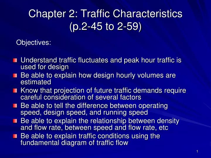
Chapter 2: Traffic Characteristics (p.2-45 to 2-59)

1. Chapter 2: Traffic Characteristics(p.2-45 to 2-59) • Understand traffic fluctuates and peak hour traffic is used for design • Be able to explain how design hourly volumes are estimated • Know that projection of future traffic demands require careful consideration of several factors • Be able to tell the difference between operating speed, design speed, and running speed • Be able to explain the relationship between density and flow rate, between speed and flow rate, etc • Be able to explain traffic conditions using the fundamental diagram of traffic flow Objectives:

2. 2.3 Traffic Characteristics • Traffic (2.3.1 General Considerations)  the most important indicator of the service for which the improvement is being made.  It directly affects the geometric features of the design • Traffic volume • Speed • (2.3.2) ADT vs. AADT  What are these? Do you know the difference? Which one requires adjustments by such adjustment factors as the seasonal, monthly, or day of week? And, why do you need adjustments?  Is ADT good for geometric design? An ‘average’ means that there is more traffic 50% of the time, and less traffic 50% of the time. Since traffic fluctuates this is not a good parameter for design. It may be good for planning purposes.

3. Variations in traffic (2.3.2 Volume)

4. AADT at the Moark Junction (2012) Visit www.udot.utah.gov.

5. 2009 count data at the Moark Junction

6. Moark Junction Traffic Dayly Distribution (2009 data)

7. Moark Junction: Peaking characteristics during peak hour

8. 2.3.2 Peak-Hour Traffic • Traffic volumes for an interval of time shorter than a day more appropriately reflect the operating conditions that should be used for design if traffic is to be properly served. • Design for rush-hour periods; then, you can take care of other periods easily. A practical and adequate time period is one hour. • Determine which of the rush-hour traffic volumes should be used for design. Using the max hourly volume may be wasteful.

9. 2.3.2 Peak-Hour Traffic (cont) • Based on this idea and a trend found in the relationship between hourly volume as a % of ADT and the number of hours in one year, use of 30 HV became accepted. 29 hours of total 8760 hours/year, this design value will be exceeded (0.33% - not bad).  See Figure 2-28. This 30 HV applies to both rural and urban roads (Rural – about 15%; Urban about 8 to 12%) • On rural roads with average fluctuation in traffic flow, 30 HV approximates 15% of ADT. • The max hourly volume is about 25% of ADT. (25% - 15%)/15% = 67%. The 30 HV is exceeded by the max hourly volume by 67%. If you used the max hourly volumes, you would have a luxurious facility. • Consider 170th HV, which is about 11.5%. (15%-11.5%)/15% = 23%. 170 HV is about 23% less than 30 HV. Figure 2-28

10. Dealing with Recreational Roads • How do we deal with recreational roads? See the figure on the right. • The max hourly volume is almost twice as much as the 30HV for partially recreational routes. • Two guiding principles • Somewhat less satisfactory traffic operation during seasonal peaks – people may accept it • Severe congestion is still not acceptable • Greenbook’s suggestion  “It may be desirable to choose an hourly volume for design, which is about 50% of the volumes expected to occur during a very few hours of the design year whether or not it is equal to 30 HV.” (p.2-49 2nd paragraph)

11. 2.3.3 Directional Distribution • Design hourly volume • 2-lane 2-way highways: Total traffic in both directions • Multilane highways: Directional design hourly volume is needed (DDHV) • Note that you must have DDHV for both morning and afternoon peak hours. In reality, we have to provide discrete number of lanes, like 2, 3, 4, etc; so, we usually end up with the same number of lanes for both directions. Also, after all, design traffic demands are estimates. • Usually, we observe a facility similar to the one under design and find an estimate of directional split. DDHV = ADT * % for 30 HV * Directional Split (Near the Moark Junction, determine DDHV.)

12. 2.3.4 Composition of Traffic • Affect the design, especially trucks • For capacity computation, grouping are: • Passenger cars: all passenger cars, minivans, pick-ups, SUVs • Trucks: buses, SU trucks, combination trucks, RVs • % of truck traffic during the peak hours should be known • % of truck traffic during the peak hours are known to be less than % of truck traffic for the 24-hour periods. Why?

13. 2.3.5 Projection of Future Traffic Demand • Discussed in CEEn 565 Urban Transportation Planning • Physical life expectancies of parts of the highway are different: right of way, surfacing, pavement, bridges (superstructure, substructure) • “In a practical sense, the design volume should be a value that can be estimated with reasonable accuracy” (3rd paragraph p.2-53) – a design period of 20 years is typical.

14. 2.3.6 Speeds • Speed  one of the most important factors to the traveler in selecting alternate routes or transportation modes (higher speed, shorter travel time) • Speed is a “barometer” of convenience and economy. • 4 general conditions affecting speed besides individual drivers’ capabilities: • The physical characteristics of the highway and its roadsides • The weather • The presence of other vehicles • The speed limitation

15. 2.3.6 Types of Speed used in Traffic engineering • Operating speed The speed at which drivers are observed operating their vehicles during free-flow conditions. The 85th percentile of the distribution of observed speeds is the most frequently used measure of the operating speed associated with a particular location or geometric feature. • Running speed The speed at which an individual vehicle travel over a highway section. The running speed is the length of the highway section divided by the running time required for the vehicle to travel through the section. (Delay time is excluded.) • Travel speed  Distance/Travel Time Travel time = running time + delay

16. Types of Speed used in Traffic engineering (cont) • Design speed  the maximum safe speed that can be maintained over a specified section of highway when conditions are so favorable that the design features of the highway govern (topography, adjacent land use, functional classification). Must meet drivers’ expectation • Use 5 mph increment • Maintain 50 to 70 mph design speeds for freeways and expressways • Maintain 30 to 60 mph for urban arterials

17. Relationship between Design Speed and Average Running Speed • A greater proportion of drivers operate near or at the design speed on highways with low design speed than on highways with high design speed. (Confirm this using the Figure on the right.) • On high design speed curves the average speed is substantially below the design speed and approaches the average spot speed found on long stretches of tangent alignment (i.e. People slow down on curves.). • As traffic volume is approaching the capacity of the highway, the average running speed decreases because of interference among vehicles. This figure was removed from the 2004 and 2011 editions.

18. Speed data on US 89

19. 2.3.7 Speed and Flow Rate • Speed is insensitive to flow rate for a certain range of flow rate (see the figure on the right)  Speed is not a good parameter for evaluating level of service (quality of flow ) of the highway. (Do you remember what MOE is used?) • As flow approaches capacity, speed drops off at a sharp rate. This figure does not exist in 2004 and 2011 edition.

20. HCM2010 Basic Speed-Flow Curves Freeways Multilane Highways

21. Flow-density relationships Flow = (density) x (Space mean speed) Space mean speed = (flow) x (Average space headway) where Average space headway = (SMS) x (Average time headway) where

22. Fundamental diagram of traffic flow (SMS vs. density & SMS vs. flow) uf uf Uncongested flow SMS (u) SMS (u) Congested flow 0 0 kj qmax Density (k) Flow (q) SMS vs. density SMS vs. flow

23. Fundamental diagram of traffic flow (flow vs. density) Optimal flow or capacity,qmax Mean free flow speed, uf Optimal speed, uo Flow (q) Speed is the slope. u = q/k Uncongested flow Congested flow Jam density, kj Optimal density, ko Density (k)