Download
1 / 28
280 likes | 448 Views
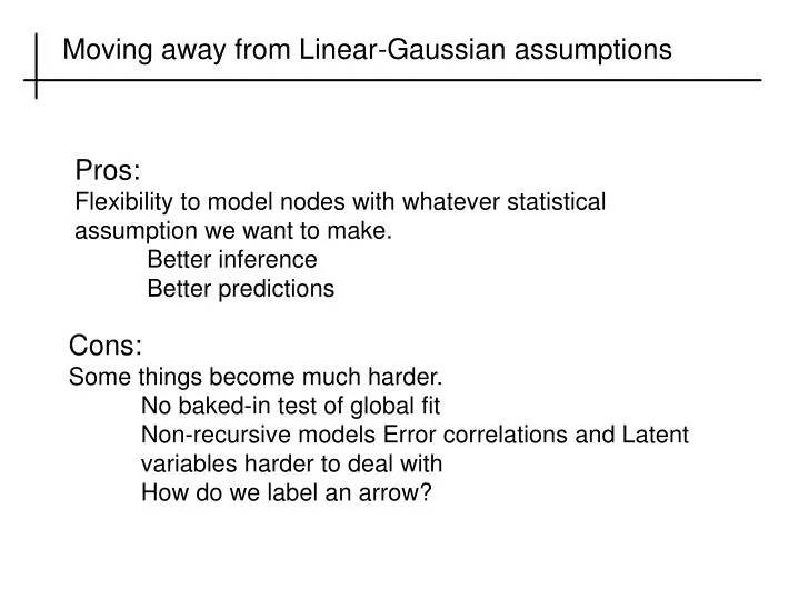
Moving away from Linear-Gaussian assumptions. Pros: Flexibility to model nodes with whatever statistical assumption we want to make. Better inference Better predictions . Cons: Some things become much harder. No baked-in test of global fit

E N D
Moving away from Linear-Gaussian assumptions Pros: Flexibility to model nodes with whatever statistical assumption we want to make. Better inference Better predictions Cons: Some things become much harder. No baked-in test of global fit Non-recursive models Error correlations and Latent variables harder to deal with How do we label an arrow?
Causal Effects in Non-linear models: How big is the effect? age firesev
The Logic of Graphs: Conditional Independences, Missing link & Testable implications How do we test structure of the model without Var-Cov matrix? For directed, acyclic models where all nodes are observed, Vi⏊Non-Child(Vj)|Pa(Vi,Vj) The residuals of each pair of nodes not connected by a link should be independent. Each missing link represents a local test of the model structure Individual test results can be combined using Fisher’s C to give a global test of structure. x y1 y2 y3
The Logic of Graphs: Conditional Independences, Missing link & Testable implications How do we test structure of the model without Var-Cov matrix? How many implied CI there? N(N-1)/2-L Where N= number of nodes L=number of links x y1 y2 y3
Strategy for local estimation analysis Create a causal graph Model all nodes as functions of variables given by graph (using model selection of pick functional form) Evaluate all conditional independences implied by graph using model residuals If conditional independence test fails modify graph and goto 2
Generalized Linear Models – 3 components A probability distribution from the exponential family Normal, Log-Normal, Gamma, beta, binomial, Poisson, geometric A Linear predictor A Link function g such that Identity, Log, Logit, Inverse
California wildfires example hetero distance rich abio age firesev cover 7
California wildfires example hetero distance rich abio age firesev cover 8
A. Submodel – it’s causal assumptions and testable implications. Causal Assumptions: dist age age firesev firesev cover cover rich dist rich Implied Conditional Independences: firesev⏊ dist | (age) cover ⏊ dist | (firesev) cover ⏊ age | (firesev) rich ⏊ age | (cover,dist) rich ⏊ firesev | (cover,dist)
A. Functional Specification I – Models of Uncertainty VariablePotential valuesProb. Dist. age {0,1,2,3,…} Negative Binom rich {0,1,2,3,…} Negative Binom firesev (0, ∞) Gamma cover (0, ∞) Gamma
B. Modeling the Nodes - Age dist >library(MASS) >a1.lin<-glm.nb(age~distance,data=dat) >a1.q<-glm.nb(age~distance+I(distance^2),…) age >curve(exp(p.l[1]+p.1[2]*x),from=0,to=100,add=T) >curve(exp(p.q[1]+p.q[2]*x+p.q[3]*x^2),from=0,to=100,add=T,lty=2) > AICtab(a1.lin,a1.q,weights=T) dAICdf weight a1.q 0.0 4 0.99662 a1.lin 11.4 3 0.00338
B. Modeling the Nodes - Firesev age firesev >f.lin<-glm(firesev~age,family=Gamma(link="log"),…) >curve(exp(p.f.lin[1]+p.f.lin[2]*x),from=0,to=100,add=T)
B. Modeling the Nodes - Firesev age firesev >f.sat<-glm(firesev~I(1/age),family=Gamma(link="inverse"),…) >curve(1/p.f.sat[2]*x/(1+1/p.f.sat[2]*p.f.sat[1]*x),from=0, to=65,add=T,lty=2)
B. Modeling the Nodes - Firesev age firesev > AICtab(f.lin,f.sat,weights=T) dAICdf weight f.sat 0.0 3 1 f.lin 16.2 3 <0.001
B. Modeling the Nodes - Cover firesev cover >c.lin<-glm(cover~firesev,family=Gamma(link=log),…) >curve(exp(p.c[1]+p.c[2]*x),from=0,to=9,add=T,lwd=2)
B. Modeling the Nodes - Richness dist firesev cover >r.lin<-glm.nb(rich~distance+cover,data=dat) >r.q<-glm.nb(rich~distance+I(distance^2)+cover,…) > AICtab(r.lin,r.q,weights=T) dAICdf weight r.q 0.0 5 0.99767 r.lin12.1 4 0.00233
C. Testing the conditional independences Implied Conditional Independences: firesev⏊ dist | (age) cover ⏊ dist | (firesev) cover ⏊ age | (firesev) rich ⏊ age | (cover,dist) rich ⏊ firesev | (cover,dist) Method for testing conditional indepedences: For each implied conditional independence statement: 1. Hypothesize that a link between the variables exists Quantify the evidence that the link explains residual variation in the variable chosen as the response.
C. Testing the conditional independences What we need: List of all implied conditional independences Residuals for all fitted nodes >source(‘glmsem.r') >fits=c("a1.q","f.sat","c.lin","r.q") >stuff<-get.stuff.glm(fits,dat) get.stuff.glm returns: R^2 for each node ($R.sq) Estimated Causal Effect*(over obs. range) ($est.causal.effects) Graph implied condition independences ($miss.links) Predicted values for each node ($predictions) Residuals for each node ($residuals) Matrix of links in the graph ($links) Matrix of prediction equations ($pred.eqns)
C. Testing the conditional independences >nl.detect3(dat,stuff$residuals,stuff$miss.links) $p.vals distance-firesevdistance-cover age-cover age-rich firesev-rich 0.058 0.252 0.523 0.872 0.134 $fisher.c [1] 14.04139 $d.f [1] 10 $fisher.c.p.val [1] 0.1711122
D. Check Model - Residuals >pairs(stuff$residuals)
D. Check Model- Parameter Estimates >sapply(fits,function(x)summary(get(x))$coefficients) $a1.q Estimate Std. Error z value Pr(>|z|) (Intercept) 3.4600063194 8.944635e-02 38.682476 0.0000000000 distance -0.0228871119 5.925116e-03 -3.862728 0.0001121277 I(distance^2) 0.0002595776 6.729042e-05 3.857571 0.0001145194 $f.sat Estimate Std. Error t value Pr(>|t|) (Intercept) 0.150971 0.01325182 11.39247 5.264449e-19 I(1/age) 1.427400 0.26099889 5.46899 4.189435e-07 $c.lin Estimate Std. Error t value Pr(>|t|) (Intercept) 0.213267 0.1382210 1.542942 1.264334e-01 firesev-0.132441 0.0284891 -4.648832 1.166142e-05 $r.q Estimate Std. Error z value Pr(>|z|) (Intercept) 3.4603244955 7.030880e-02 49.216093 0.000000e+00 distance 0.0164087246 3.150035e-03 5.209060 1.897993e-07 I(distance^2)-0.0001408172 3.540241e-05 -3.977617 6.960945e-05 cover 0.2361592759 8.581527e-02 2.751949 5.924170e-03
D. Check Model- Print Resulting Graph #requires graphviz and {PNG} >glmsem.graph(stuff)
E. Run a Query (intervention) new.dat<-dat new.dat[,'age']<-2 dat.int<-calc.intervention.glm(fits,stuff $links,"age",new.dat)
Discussion Get glmsem.r and these slides and R code for exmplat: www.msu.edu/~schoolm4/Code_and_More.html