Download
1 / 50
550 likes | 726 Views
Explore Cook-Toom and Winograd algorithms for fast convolution. Learn algorithmic strength reduction and polynomial multiplication techniques. Reduce complexity with examples and implementation insights.

E N D
Chapter 8 FastConvolution • Introduction • Cook-Toom Algorithm and Modified Cook-Toom Algorithm • Winograd Algorithm and Modified WinogradAlgorithm • IteratedConvolution • CyclicConvolution • Design of Fast Convolution Algorithm byInspection 2
Introduction • Fast Convolution: implementation of convolution algorithm using fewer multiplication operations by algorithmic strengthreduction • Algorithmic Strength Reduction: Number of strong operations (such as multiplication operations) is reduced at the expense of an increase in the number of weak operations (such as addition operations). These are bestsuited for implementation using either programmable or dedicatedhardware • Example: Reducing the multiplication complexity in complexnumber multiplication: – Assume (a+jb)(c+dj)=e+jf, it can be expressed using the matrix form, which requires 4 multiplications and 2additions: da ec fd cb – However, the number of multiplications can be reduced to 3 at the expense of3 extraadditionsbyusing:acbd a(cd)d(ab) adbcb(cd)d(ab) 3
– Rewrite it into matrix form, its coefficient matrix can be decomposed as the product of a 2X3(C), a 3X3(H)and a 3X2(D)matrix: cd 0 01 0 0 c d 0 0 0 1 se1 1 00 1aCHDx f0 1 b d 1 1 • Where C is a post-addition matrix (requires 2 additions), D is a pre-addition matrix (requires 1 addition), and H is a diagonal matrix (requires 2 additions to get its diagonalelements) • – So, the arithmetic complexity is reduced to 3 multiplications and 3 additions (not including the additions in Hmatrix) • In this chapter we will discuss two well-known approaches to the design of fast short-length convolution algorithms: the Cook-Toom algorithm(based on Lagrange Interpolation) and the Winograd Algorithm (based on the Chinese remainder theorem) 4
Cook-ToomAlgorithm • A linear convolution algorithm for polynomial multiplication based on the Lagrange InterpolationTheorem • Lagrange InterpolationTheorem: Let0,....,n be asetof n 1distinct points, and let f ( i ) , for i f (p) = 0, 1,…,n begiven.Thereisexactlyonepolynomial of degree n orless thathasvalue f ( i )when evaluated at i for i = 0, 1, …, n. It is givenby: (pj) n f(p)f() ji () i i0 i j ji 5
The application of Lagrange interpolation theorem into linear convolution ConsideranN-pointsequenceh h0,h1 ,...,hN1 xx0 ,x1,...,xL1. andanL-pointsequenceThelinear convolutionofhandx can be expressed in terms ofpolynomial multiplicationasfollows: s(p)h(p)x(p) where pN 1 pL 1 h ( p) h x ( p ) x ... h1 p h0 N 1 ...x p x L1 1 0 pL N 2 s ( p ) s ...s p s LN2 1 0 LN 2 Theoutputpolynomial s (p) hasdegree andhas LN 1 differentpoints. 6
(continued) • s( p) can be uniquely determined by its values at L N 1 0,1,...,LN2 L N 1 differentpoints.Letbe for i 0,1,..., LN 2are different realnumbers.If s(i) s(p) known, then theoremas: can be computed using the Lagrangeinterpolation ( p j ) LN2 i0 ji s( p) s( ) () i i j ji Itcanbeprovedthatthisequationistheuniquesolutiontocomputelinear s(i), s(p) convolutionforgiventhevaluesoffor i 0,1,..., LN 2. 7
Cook-Toom Algorithm (AlgorithmDescription) • ChooseLN1differentrealnumbers0,1,LN2 • 2. Compute h(i) and x(i ) , for i 0,1,, L N 2 • 3. Compute s( i ) h(i ) x(i ) , for i 0,1,, L N 2 • (pj) LN2 s(p)s(i ) ji (ij) ji s(p) 4. Compute byusing i0 • AlgorithmComplexity • The goal of the fast-convolution algorithm is to reduce the multiplication complexity. So, if i `s (i=0,1,…,L+N-2) are chosen properly, the computation in step-2 involves some additions and multiplications by smallconstants • The multiplications are only used in step-3 to compute s(i). So, only L+N-1 multiplications areneeded 8
By Cook-Toom algorithm, the number of multiplications is reduced from O(LN) to L+N-1 at the expense of an increase in the number ofadditions • An adder has much less area and computation time than a multiplier. So, the Cook-Toom algorithm can lead to large savings in hardware (VLSI) complexity and generate computationally efficientimplementation • Example-1: (Example 8.2.1, p.230) Construct a 2X2 convolution algorithm using Cook-Toom algorithm with={0,1,-1} • – Write 2X2 convolution in polynomial multiplication formas s(p)=h(p)x(p),where h( p) h0 h1p x( p) x0 x1p s(p)s s p s p2 0 1 2 – Direct implementation, which requires 4 multiplications and 1 additions, can be expressed in matrix form asfollows: h0 s0 0x s h 0 h 1 1 0 x 1 s0h 2 1 9
Example-1(continued) • – Next we use C-T algorithm to get an efficient convolutionimplementation with reduced multiplicationnumber 0 0, 1 1, 2 2, h(0)h0, x( 0 ) x0 h (1 ) h0 h1 , h( 2 ) h0h1 , x( 1 ) x0 x1 x( 2 ) x0x1 • Then, s(0), s(1), and s(2) are calculated, by using 3 multiplications,as • s(0)h(0)x(0) s(1)h(1)x(1) s(2)h(2)x(2) • From the Lagrange Interpolation theorem, weget: ( p 1 )( p 2) ( p 0 )( p 1) s(p) s( ) s ( ) 0 1 ()( ) ( 1 0 )( 1 2) 0 1 0 2 ( p 0 )( p 1 ) ( 2 0 )( 2 1) s ( 2) ) s ( 1 ) s ( 2 )) s() p ( s ( 1 ) s ( 2 ) ) p 2 ( s ( 0 0 2 2 s 0 ps 1p s 2 2 10
Example-1(continued) • – The preceding computation leads to the following matrixform 1 0 0 s ( 0 ) 1 1s() 1 1 1 s ( 2) 2 1 0 0 h ( 0 ) 0 1 10 1 1 0 1 0 0 1 1 1 s 0 s 0 2 1 1 s 2 0 0 x ( ) h ( 2) 2x ( 2 ) 0 0 0 x ( 0 ) h() 2 1 0 1 1 0 0 h0 1 0 x 1 0 10 (h h ) 2 1 x 0 1 1 1 0 0 (h h) 21 1 0 1 – The computation is carried out as follows (5 additions, 3multiplications) h0 h1, h0 h1 1. H0h0, H 2. X 0 x0, 3. S 0 H 0 X0 , 4. s0 S 0, (pre-computed) H 1 2 2 2 X 1 x0 x1, S1 H 1 X1, s1 S1 S 2, X 2 x0 x1 S 2 H 2 X2 s2 S0 S1 S2 11
(Continued): Therefore, this algorithm needs 3 multiplications and 5 additions (ignoring the additions in the pre-computation ), i.e., thenumber of multiplications is reduced by 1 at the expense of 4 extraadditions • Example-2, please see Example 8.2.2 of Textbook(p.231) • Comments • Some additions in the preaddition or postaddition matrices can be shared. So, when we count the number of additions, we only count one instead of two or three. • If we take h0, h1 as the FIR filter coefficients and take x0, x1 as the signal (data) sequence, then the terms H0, H1 need not be recomputed each time the filter is used. They can be precomputed once offline and stored. So, we ignore these computations when counting the number of operations • From Example-1, We can understand the Cook-Toom algorithm asa matrix decomposition. In general, a convolution can be expressed in matrix-vector forms as h0 s0 or 0x s T x s h 0 h 1 0 1 x 1 s0h 2 1 12
– Generally, the equation can be expressedas sTxCHDx • Where C is the postaddition matrix, D is the preaddition matrix, and H is a diagonal matrix with Hi, i = 0, 1, …, L+N-2 on the maindiagonal. • Since T=CHD, it implies that the Cook-Toom algorithm provides a way to factorize the convolution matrix T into multiplication of 1postaddition matrix C, 1 diagonal matrix H and 1 preaddition matrix D, such that the total number of multiplications is determined only by the non-zero elements on the main diagonal of the diagonal matrixH • Although the number of multiplications is reduced, the number of additions has increased. The Cook-Toom algorithm can be modifiedin order to further reduce the number ofadditions 13
Modified Cook-ToomAlgorithm • The Cook-Toom algorithm is used to further reduce the numberof addition operations in linearconvolutions Defines'(p)s(p)SL pLN 2 . Notice thatthe N2 L N2 and SLN2 degreeof s( p)is is its highest order • coefficient. Therefore the degree ofs'(p) isLN3. • Now consider the modified Cook-ToomAlgorithm 14
Modified Cook-ToomAlgorithm • ChooseLN2differentrealnumbers0,1,LN3 Computeh()andx(),fori0,1,,LN3 2. 3. 4. i i Computes()h()x(),fori0,1,,LN3 i i i LN2 i 0,1, ,LN3 Computes'(i)s(i)sLN2i ,for (pj) LN2 ji s'(p) s'() () s'(p) i 5. Compute byusing i0 i j ji LN2 Computes(p)s'(p)sLN2p 6. 15
Example-3 (Example 8.2.3, p.234) Derive a 2X2 convolution algorithm using the modified Cook-Toom algorithm with={0,-1} s'(p)s(p)hxp2 Consider the Lagrange interpolation for at 11 0,1 . 0 1 s'()h()x()hx2 First,find i i h(0) h0, 1 1 i x(0) x0 x(1)x0x1 i 0 0, 1 1, h(1)h0h1, – and • s'() h() x( ) h x 2 hx • 0 0 0 1 1 0 0 0 • s'() h() x() h x 2 (h h)(x x ) hx • 1 1 1 1 1 1 0 1 0 1 11 • Which requires 2 multiplications (not counting the h1x1 multiplication) • – Apply the Lagrange interpolation algorithm, weget: (p) (p) s'(p)s'() s'() 1 0 0 1 (01) () 1 0 s'(0)p(s'(0)s'(1)) Chap.8 16
Example-3(cont’d) • Therefore, • Finally, we have the matrix-formexpression: s(p)s'(p)hxp2 s s p s p2 1 1 0 1 2 1 0 0s ' ( 0 ) 1 0 s ' ( 0 0 1 1 0 1 1 s ( 0 0 0 1 1s() s 0 s 1 ) 1 1 h1 x1 – Noticethat s 2 s ' ( 0 ) 0 s ( 0 ) ) s '( ) 0 1 h1x1 1 – Therefore: 1 h1x1 0 1 0 0 s01 01 0 s(0) s 1 1 1 s 2 x 1 1 1 0 0 0 0 h h 0 1 1 x 0 1 1 10 0 h0 1 1
Example-3(cont’d) • – The computation is carried out as the follows: • (pre-computed) • – The total number of operations are 3 multiplications and 3additions. • Compared with the convolution algorithm in Example-1, the numberof addition operations has been reduced by 2 while the number of multiplications remains thesame. • Example-4 (Example 8.2.4, p. 236 ofTextbook) • Conclusion: The Cook-Toom Algorithm is efficient as measured by the number of multiplications. However, as the size of the problem increases, it is not efficient because the number of additions increases greatly if takes values other than {0, 1, 2, 4}. This may result in complicated pre-addition and post-addition matrices. For large-size problems, the Winograd algorithm is moreefficient.
WinogradAlgorithm • The Winograd short convolution algorithm: based on the CRT (Chinese Remainder Theorem) ---It’s possible to uniquely determine a nonnegative integer given only its remainder with respect to the given moduli, provided that the moduli are relatively prime and the integer is known to be smaller than the product of themoduli • Theorem: CRT forIntegers c R c c is divided by mi ),for arerelativelyprime,then Given (represents the remainderwhen i m i i0,1,...,k,mi wherearemoduliand k cciNiMimodM ,where k M m Mi M mi i ,, i0 i0 NiMinimiGCD(Mi,mi)1,provided and Ni is the solution of that0cM
Theorem: CRT forPolynomials c(i) (p)R (p)c( p), m( i) m(i)(p) Given fori=0, 1, …,k, where are k (i) c(i)(p)N(i)(p)M relatively prime, then c( p) (p)modM(p), where i0 k m(i) (p),M(i)(p)M(p)m(i)(p),andN(i)(p)isthe solution of M(p) i0 • N(i)(p)M(i)(p)n(i)(p)m(i)(p)GCD(M(i)(p),m(i)(p))1 Provided that the degree of c(p) is less than the degree of M ( p) • Example-5 (Example 8.3.1, p.239): using the CRT for integer,Choose moduli m0=3, m1=4, m2=5.Then Then: M m0m1m2 60,and M iM mi. – whereNi that thei CD algorithm.Given c.
Example-5(cont’d) • – The integer c can be calculatedas k cciNiMimodM(20c015c124c2)mod60 i0 – Forc=17, c0 R3(17)2, c1 R4(17)1, c2 R5(17) 2 • c(202151242)mod60103mod6017 • CRT for polynomials: The remainder of a polynomial with regard tomodulus • pi f ( p), where deg( f ( p)) i 1, can be evaluated bysubstitutingpi by • f ( p) in thepolynomial • Example-6 (Example 8.3.2,pp239) R 5x23x55(2)23(2)519 (a). (b). (c).R x2 R 5x23x55(2)3x53x5 x22 5x 3x5 5( 2 x2)3x52x5 x2x2
WinogradAlgorithm • 1. Choose a polynomial m( p) with degree higher than the degree of h(p)x(p)and factoritintok+1 relativelyprimepolynomials withreal coefficients,i.e.,m(p)m(0)(p)m(1)(p)m(k)(p) • 2. Let M ( i) ( p) m(p) m(i)(p).UsetheEuclideanGCDalgorithmto solveN(i)(p)M(i)(p)n(i)(p)m(i)(p)1forN(i)(p). • 3. Compute:h(i)(p)h(p)modm(i)(p), x(i)(p)x(p)modm(i)(p) • for i 0,1,,k • – 4. Compute:s(i)(p)h(i)(p)x(i)(p)modm(i)(p), for i 0,1,,k – 5. Computes(p) byusing: s(p)s(i)(p)N(i)(p)M(i)(p)modm(i)(p) i0 k
Example-7 (Example 8.3.3, p.240) Consider a 2X3 linear convolution as in Example 8.2.2. Construct an efficient realization using Winogradalgorithm with m( p) p( p 1)( p2 1) • Let: • Construct the following table using the relationships M ( i) ( p) m(p) m(i)(p) m(0)(p)p, m(1) ( p) p 1, m( 2) ( p) p2 1 and for i 0,1,2 N(i)(p)M(i)(p)n(i)(p)m(i)(p)1 Compute residues from h( p) h hp, x( p)x x p xp2: – 0 1 0 1 2 h( 0) ( p) h , x(0)(p)x 0 0 h(1) ( p)h h, 0 1 x (1) ( p)x x x 0 1 2 h( 2) ( p)h hp, 0 1 x( 2) ( p) (x0 x2 ) x1 p
Example-7(cont’d) s ( 0 ), (1) s(0)(p)hx s (1) ( p)(h h)(x x x ) s 0 1 0 1 2 0 0 0 0 s(2)(p)(h hp)((x x ) x p) mod( p 2 1) 0 1 0 2 1 s( 2 ) p h(x x ) h x (h x h(x x )) p s (2) 0 0 2 1 1 0 1 1 0 2 0 1 • Notice, we need1 multiplicationfors(0)(p),1 fors(1)(p),and 4fors(2)(p) • However it can be further reduced to 3 multiplications as shownbelow: 0 0 h0 h1 0 0 x 0 x1 x 2 0 h0 ( 2 ) 1 0 1 1 1 0 s x 0 x2 0 ( 2) s 1 0 h h x 1 0 1 – Then: 2 s(p)s(i)(p)N(i)(p)M(i)(p)modm(i)(p) i0 s (p)(p p p 1) S (1 ) ( p ) ( p3 p) S ( 2 ) ( p ) ( p3 2 p 2 p) (0) 3 2 2 2 mod( p 4 p 3 p 2 p)
Example-7(cont’d) • – Substitutes(0)(p), s(1)(p), s(2)(p)intos(p)toobtainthefollowing table – Therefore, wehave s 1 0 0 s 1 1 1 0 2 1 1 ( 0) 0 s 0 0 (1) 1 s 1 2 0 1 ( 2 ) 1s s 1 0 2 2 0 1s s ( 2) 1 1 3 2 1
Example-7(cont’d) – Noticethat ( 0) 0 0 h0 h1 h x 2 0 0 s 0 x x 1s 0 1 2 0 0 0 (1) 20 h0 2 0 0 2 0 0 x • x x 1s h1 h0 2 0 0 1 ( 2) 2 0 0 0 x x 0 0 1 1 0 0 2 ( 2) s 1 21 0 h 0 h1 2 x 1 – So, finally wehave: 0 0 h0 2 0 0 0 0 0 h1 h0 2 0 0 0 0 h0 0 0 h 0 h1 1 0 0 0 0 1 1 2 1 1 1 0 2 0 1 0 0 1 1 s 0 2 0 0 0 s 1 0 s 2 2 0 s h 0 h1 3 0 0 2 0 1 1 1 1 x1 0 1 1 0 1 1 x 0 1 1x 2 0 0
Example-7(cont’d) • In this example, the Winograd convolution algorithm requires 5 multiplications and 11 additions compared with 6 multiplications and2 additions for directimplementation • Notes: • The number of multiplications in Winograd algorithm is highlydependent on the degree of each m( i ) ( p). Therefore, the degree of m(p) should be as small as possible. • More efficient form (or a modified version) of the Winograd algorithm can be obtained by letting deg[m(p)]=deg[s(p)] and applying the CRTto s ' ( p) s ( p) hN ( p) • 1 x L 1m
Modified WinogradAlgorithm • 1. Choose a polynomial m( p) with degree equal to the degree of s( p) and factor it into k+1 relatively prime polynomials with realcoefficients, i.e., m(p)m(0)(p)m(1)(p)m(k)(p) • 2. Let M ( i) ( p) m(p) m(i)(p),use theEuclideanGCDalgorithmto solveN(i)(p)M(i)(p)n(i)(p)m(i)(p)1forN(i)(p). h(i)(p)h(p)modm(i)(p), x(i)(p)x(p)modm(i)(p) for i 0,1,,k – 3.Compute: – – 5. Compute s' ( p) byusing: 4. Compute:s'(i)(p)h(i)(p)x(i)(p)modm(i)(p), for i0,1,,k k s'(p)s'(i)(p)N(i)(p)M(i)(p)modm(i)(p) i0 s(p)s'(p)hN1xL1m(p) – 6.Compute
Example-8 (Example 8.3.4, p.243 ): Construct a 2X3 convolution algorithm using modified Winograd algorithm withm(p)=p(p-1)(p+1) m(0)(p)p, m(1) ( p) p1, m(2)(p)p1 • Let • Construct the following table using the relationships M ( i) ( p) m(p) m(i)(p) and N(i)(p)M(i)(p)n(i)(p)m(i)(p)1 • hp, x( p)x x p xp2: 0 1 2 – Compute residues from h( p) h 0 1 h( 0) ( p) h, x(0)(p)x 0 0 h(1) ( p)h h, 0 1 x(1) ( p)x x x 0 1 2 h( 2) ( p)h h, 0 1 x( 2) ( p) x0 x1 x 2 s'( 0) ( p) h x, s'(1) ( p)(h h)(x x x ), 0 1 0 1 2 0 0 s'( 2) ( p)(h h)(x x x ) 0 1 0 1 2
Example-8(cont’d) • – Since the degree of m( i ) ( p) is equal to 1, s'( i) ( p) is a polynomial of degree 0 (a constant). Therefore, wehave: • s(p)s'(p)h1x2m(p) s'(0) (p2 1) (1) (2) 2 2 3 (p p) (p p) h x(p p) S' S' 12 2 2 (0)s'(1)s'(2) 2 (0) 3 (1) (2) s' p( hx)p(s' ) p (h x) s' s' 1 2 2 2 12 2 2 – The algorithm can be written in matrix formas: s'( 0 ) 1 0 0 0 1 1 1 s 1 1 1 0 0001 s0 s'(1) s 0 1 2 s '( 2) 2 2 s3 h1 x2
Example-8(cont’d) • – (matrixform) 0 0 h0 h1 1 0 0 0 h0 0 1 1 0 h0 h1 1 1 1 0 0 0 0 1 0 0 1 1 1 1 1 0 0 0 s0 s 0 0 1 1 0 h1 2 0 0 s 0 2 2 0 1 0 s3 x 1 0 x 1 x 1 2 – Conclusion: this algorithm requires 4 multiplications and 7additions
IteratedConvolution • Iterated convolution algorithm: makes use of efficientshort-length convolution algorithms iteratively to build longconvolutions • Does not achieve minimal multiplication complexity, but achievesa • good balance between multiplications and additioncomplexity • Iterated Convolution Algorithm(Description) • 1. Decompose the long convolution into several levels ofshort convolutions • 2. Construct fast convolution algorithms for shortconvolutions • 3. Use the short convolution algorithms to iteratively(hierarchically) implement the longconvolution • Note: the order of short convolutions in the decomposition affectsthe complexity of the derived longconvolution
Example-9 (Example 8.4.1, pp.245): Construct a 4X4 linear convolution algorithm using 2X2 shortconvolution h( p)h h p h p2 hp3, x( p)x x p x p 2 xp3 – Let 0 1 2 3 0 1 2 3 and s( p) h( p)x(p) – First, we need to decompose the 4X4 convolution into a 2X2convolution – h'0 ( p) h0 h1 p, x'0 ( p) x0 x1p, – Then, wehave: h'1 ( p) h2 h3 p x'1 ( p) x2 x3p Define h(p)h'(p)h'(p)p2, 0 1 i.e.,h(p)h(p,q)h'0(p)h'1(p)q x(p)x'(p)x'(p)p2, i.e.,x(p)x(p,q)x'(p)x'(p)q 0 1 0 1 s(p)h(p)x(p)h(p,q)x(p,q) h'0(p)h'1(p)qx'0(p)x'1(p)q h' (p)x' (p)h'(p)x'(p)h'(p)x'(p) 2 q h' ( p)x' (p)q 0 0 0 1 1 0 1 1 s' (p)s'(p)qs' (p)q2s(p,q) 0 1 2
Example-9(cont’d) • Therefore, the 4X4 convolution is decomposed into two levels ofnested 2X2convolutions • Let us startfrom the first convolutions'0(p)h'0(p)x'0(p), we have: • h'0(p)x'0(p)h'0x'0(h0h1p)(x0x1p) (hh ) (x x)hx h x 2 hx hxp p 0 0 1 1 0 1 0 1 0 0 11 – We have the following expression for the thirdconvolution: s'2(p)h'1(p)x'1(p)h'1x'1(h2h3p)(x2x3p) hx h x p2p(h h )(x x ) hx h x 2 2 3 3 2 3 2 3 2 2 33 – For the second convolution, we get the followingexpression: s'1(p)h'0(p)x'1(p)h'1(p)x'0(p)h'0x'1h'1x'0 (h' h' ) (x' x' ) h' x' h' x' 0 1 0 1 0 0 1 1 :addition :multiplication
Example-9(Cont’d) (h'0h'1)(x'0x'1), we have the following expression: • For (h'0h'1)(x'0x'1)(h0h2)p(h1h3)(x0x2)p(x1x3) (hh)(xx)p2(hh)(xx) 0 2 0 2 1 3 1 3 p[(h0h1h2h3)(x0x1x2x3) (h0h2)(x0x2)(h1h3)(x1x3)] This requires 9 multiplications and 11additions – If we rewrite the three convolutions as the following expressions, then we can get the following table (see the nextpage): h' x' apa p2a 0 0 1 2 3 h' x' bpb p2b 1 1 1 2 3 h' h' x' x'c pc • p2c 0 1 0 1 1 2 3
Example-9(cont’d) Total 8 additionshere – Therefore, the total number of operations used in this 4X4iterated convolution algorithm is 9 multiplications and 19additions
CyclicConvolution • Cyclic convolution: also known as circularconvolution • • Letthefiltercoefficientsbehh0,h1,,hn1,andthedata xx0,x1,,xn1. sequencebe – The cyclic convolution can be expressedas x h(p)x(p)mod(p1) n s(p)h n – The output samples are givenby n1 hi k xk , si i 0,1,,n 1 k0 • whereikdenotesikmodn • The cyclic convolution can be computed as a linear convolution reduced by modulo pn 1. (Notice that there are 2n-1 different output samples for this linear convolution). Alternatively, the cyclic convolution can be computed using CRT with m( p) pn 1, which is muchsimpler.
Example-10 (Example 8.5.1, p.246) Construct a 4X4 cyclicconvolution 1(p1)(p1)(p21) algorithm using CRTwith m(p)p4 • Let h( p)h h p h p2 h p3, • Let • Get the following table using the relationships M ( i) ( p) m(p) m(i)(p) x( p)x x p x p 2 xp3 0 1 2 3 0 1 2 3 m( 0 ) ( p)p 1, m (1) ( p) p1, m(2)(p)p21 and N(i)(p)M(i)(p)n(i)(p)m(i)(p)1 – Compute the residues h(0)(p)h hh h h ( 0), 0 1 2 3 0 h(1) ( p)h hh h h (1), 0 1 2 3 0 (2)h(2)p h( 2) ( p)h h h h p h 0 2 1 3 0 1
Example-10(cont’d) :multiplication (0), (1), x(0)(p)x x x x x 0 1 2 3 0 x (1) ( p)x x x x x 0 1 2 3 0 ( 2 )x ( 2) p x(2)(p)x x x x p x 0 2 1 3 0 1 s(0)(p)h(0)(p)x(0)(p)h(0)x(0)s(0), 0 0 0 s(1)(p)h(1)(p)x(1)(p)h(1)x(1)s(1), 0 0 (2) 0 s1 ph (p)x (p)mod(p1) (2)(2) (2) (2) 2 s ( p) s0 h x x p (2)(2) (2) (2) (2) (2) (2) (2) • h h x hx 0 0 1 1 0 1 1 0 – Since h h x , ( 2 ) h ( 2) x ( 2) h ( 2) x (2) (2) (2) (2) (2) (2) (2) s x x h • h 1 (2) 0 (2) 0 0 0 1 1 0 0 1 1 x x h • h s ( 2) h ( 2) x ( 2) h ( 2) x (2) (2) (2) (2) (2) x , 1 0 1 1 0 0 0 1 1 0 0 – or inmatrix-form h(2) x(2)x(2) 0 0 0 (2) 0 0 1 s 101 h(2)h(2) x(2) 0 0 s ( 2) 10 1 0 0 1 0 h(2) h(2) x(2) 1 0 0 1 1 – Computations so far require 5multiplications
Example-10(cont’d) • s(p)s(i)(p)N(i)(p)M(i)(p)modm(i)(p) – Then 2 i0 s )sp 3 2 3 2 2 2 (0) p p p1 (1) p p p1 (2) p 1 (2) p1 ( )s( )s ( 0 s(0 ) s(1) s( 2) 0 0 1 4 4 s(0)s(1)s 2 2 p p s( 0) s(1) s(2) (2) 2 • p s s s 11 4 0 2 1 3 (0) (1) (2) 1 4 0 – So, wehave 1110 1 1 0 1 1 1 0 1 1 0 1 (0) 4 0 s s 1 0 1s(1) s 4 1 0 (2) 0 (2) 1 s2 s 1 2 s s 1 3 2 1
Example-10(cont’d) • – Noticethat: 1s(0) 1 0 0 0 0 0 1 0 0 0 00101 0 1 1 0 0 0 4 0 1s(1) 4 0 (2) s 1 2 0 1s(2) 2 1 1h(0) x(0) 4 0 0 4 0 0 0 2 0 0 0 0 h 0 0 0 0 1h(1) x(1) 0 1h(2) 0 0 (2) (2) x x 0 1 x(2) (2) (2) • h 0 1 2 1 0 0 h h x(2) (2)(2) 0 1 2 0 1 1
Example-10(cont’d) • – Therefore, wehave 1 1 0 1 1 1 1 1 1 0 1 1 1 1 1 0 0 s01 1 0 s1 1 s2 s 3 h 0 h1 h 2 h3 0 0 h 0 h2 0 0 0 h 0 h 1 h 2 h3 2 0 0 0 4 0 0 h 0 h1 h 2 h3 4 0 0 h 0 h1 h 2 h 3 0 1 2 1 1 x 1 1 0
Example-10(cont’d) • This algorithm requires 5 multiplications and 15additions • The direct implementation requires 16 multiplications and 12 additions (see the following matrix-form. Notice that the cyclic convolutionmatrix is a circulantmatrix) h0 h3 h2 h1 s0x0 shhx h h 1 1 2 1 0 3 h1h0 h h s2h2 h3x2 s h h x 303 3 2 1 • An efficient cyclic convolution algorithm can often be easily extended to construct efficient linearconvolution • Example-11 (Example 8.5.2, p.249) Construct a 3X3 linear convolution using 4X4 cyclic convolutionalgorithm
Example-11(cont’d) – Let the 3-point coefficient sequence be hh0,h1,h2, and the 3-point data sequence be xx0,x1,x2 – First extend them to 4-point sequencesas: hh0,h1,h2,0, xx0,x1,x2,0 – Then the 3X3 linear convolution of h and xis h0x0 h0 x0 h2 x2 h1x0 h0x1 h1x0 h0 x1 2 0 1 1 0 2 hxhx h x h x hx 4 hx h x h x 2 0 1 1 0 2 h2x1 h1x2 h2 x1 h1x2 hx 2 2 – The 4X4 cyclic convolution of h and x, i.e. h4 x,is:
Example-11(cont’d) – Therefore, we haves(p)h(p)x(p)hxhx(p41) n 2 2 – UsingtheresultofExample-10forh4x,thefollowingconvolution algorithm for 3X3 linear convolution isobtained: 1 1 1 0 1 1 s0 1 s 1 s 2 1 1 s3 0 s 4 (continued on the nextpage)
Example-11(cont’d) h 0 h1 h2 0 h 0 h1 h2 0 4 0 4 0 0 0 0 0 0 0 0 1 1 1 1 1 1 1x 0 1 0 0 1 0 0 h 0 h1 h2 0 0 h 0 h1 h2 0 h0h2 2 0 0 0 0 2 0 0 0 h 2 2 0 1 1 x 0 1 1 1 x 2 0 0
Example-11(cont’d) • So, this algorithm requires 6 multiplications and 16 additions • Comments: • In general, an efficient linear convolution can be used to obtain an efficient cyclic convolution algorithm. Conversely, an efficient cyclic convolution algorithm can be used to derive an efficient linear convolutionalgorithm
Design of fast convolution algorithmby inspection • When the Cook-Toom or the Winograd algorithms can not generate an efficient algorithm, sometimes a clever factorization by inspection may generate a betteralgorithm • Example-12 (Example 8.6.1, p.250) Construct a 3X3 fast convolution algorithm byinspection • – The 3X3 linear convolution can be written as follows, which requires9 multiplications and 4additions h0x0 s0 s h1x0 h0x1 1 s2h2x0h1x1h0x2 s h2 x1 h1x2 h2x2 3 s4
Example-12(cont’d) • – Using the followingidentities: • s1h1x0h0x1h0h1x0x1h0x0h1x1 • s2h2x0h1x1h0x2h0h2x0x2h0x0h1x1h2x2 • s3h2x1h1x2h1h2x1x2h1x1h2x2 • – The 3X3 linear convolution can be writtenas: 1 0 s0 0 s 1 1 0 (continued on the nextpage) s 2 1 0 1 s3 0 0 s 4
Example-12(cont’d) h000 0 0 0 0 0 0 0 0 0 0 0 0 0 0 1 0 0 1 1 0 0 1 1 1 0 0 h 0 1 x 0 h 0 0 0 h h 0 0 0 0 0 0 0 1 x 2 1 0 1 x 2 0 h h 0 0 h1 0 1 1 0 0 2 h20 – Conclusion: This algorithm, which can not be obtained byusing the Cook-Toom or the Winograd algorithms, requires 6 multiplications and 10additions