Download
1 / 53
530 likes | 564 Views
Chapter 13: Query Optimization. Chapter 13: Query Optimization. Introduction Transformation of Relational Expressions Catalog Information for Cost Estimation Statistical Information for Cost Estimation Cost-based optimization Dynamic Programming for Choosing Evaluation Plans

E N D
Chapter 13: Query Optimization • Introduction • Transformation of Relational Expressions • Catalog Information for Cost Estimation • Statistical Information for Cost Estimation • Cost-based optimization • Dynamic Programming for Choosing Evaluation Plans • Materialized views
Introduction • Alternative ways of evaluating a given query • Equivalent expressions • Different algorithms for each operation
Introduction (Cont.) • An evaluation plan defines exactly what algorithm is used for each operation, and how the execution of the operations is coordinated. • Find out how to view query execution plans on your favorite database
Introduction (Cont.) • Cost difference between evaluation plans for a query can be enormous • E.g. seconds vs. days in some cases • Steps in cost-based query optimization • Generate logically equivalent expressions using equivalence rules • Annotate resultant expressions to get alternative query plans • Choose the cheapest plan based on estimated cost • Estimation of plan cost based on: • Statistical information about relations. Examples: • number of tuples, number of distinct values for an attribute • Statistics estimation for intermediate results • to compute cost of complex expressions • Cost formulae for algorithms, computed using statistics
Transformation of Relational Expressions • Two relational algebra expressions are said to be equivalent if the two expressions generate the same set of tuples on every legal database instance • Note: order of tuples is irrelevant • we don’t care if they generate different results on databases that violate integrity constraints • In SQL, inputs and outputs are multisets of tuples • Two expressions in the multiset version of the relational algebra are said to be equivalent if the two expressions generate the same multiset of tuples on every legal database instance. • An equivalence rule says that expressions of two forms are equivalent • Can replace expression of first form by second, or vice versa
Equivalence Rules 1. Conjunctive selection operations can be deconstructed into a sequence of individual selections. 2. Selection operations are commutative. 3. Only the last in a sequence of projection operations is needed, the others can be omitted. • Selections can be combined with Cartesian products and theta joins. • (E1X E2) = E1 E2 • 1(E12 E2) = E11 2E2
Equivalence Rules (Cont.) 5. Theta-join operations (and natural joins) are commutative.E1 E2 = E2E1 6. (a) Natural join operations are associative: (E1 E2) E3 = E1 (E2 E3)(b) Theta joins are associative in the following manner:(E1 1E2) 2 3E3 = E1 1 3 (E22 E3) where 2involves attributes from only E2 and E3.
Equivalence Rules (Cont.) 7. The selection operation distributes over the theta join operation under the following two conditions:(a) When all the attributes in 0 involve only the attributes of one of the expressions (E1) being joined.0E1 E2) = (0(E1)) E2 (b) When 1 involves only the attributes of E1 and2 involves only the attributes of E2. 1 E1 E2) = (1(E1)) ( (E2))
Õ = Õ Õ ( E E ) ( ( E )) ( ( E )) È q q L L 1 2 L 1 L 2 1 2 1 2 Equivalence Rules (Cont.) 8. The projection operation distributes over the theta join operation as follows: (a) if involves only attributes from L1 L2: (b) Consider a join E1 E2. • Let L1 and L2 be sets of attributes from E1 and E2, respectively. • Let L3 be attributes of E1 that are involved in join condition , but are not in L1 L2, and • let L4 be attributes of E2 that are involved in join condition , but are not in L1 L2. Õ = Õ Õ Õ ( E E ) (( ( E )) ( ( E ))) È q È È È q L L 1 2 L L L L 1 L L 2 1 2 1 2 1 3 2 4
Equivalence Rules (Cont.) • The set operations union and intersection are commutative E1 E2 = E2 E1E1 E2 = E2 E1 • (set difference is not commutative). • Set union and intersection are associative. (E1 E2) E3 = E1 (E2 E3)(E1 E2) E3 = E1 (E2 E3) • The selection operation distributes over , and –. (E1 – E2) = (E1) – (E2)and similarly for and in place of –Also: (E1 – E2) = (E1) – E2 and similarly for in place of –, but not for 12. The projection operation distributes over union L(E1 E2) = (L(E1)) (L(E2))
Transformation Example: Pushing Selections • Query: Find the names of all instructors in the Music department, along with the titles of the courses that they teach • name, title(dept_name= “Music”(instructor (teaches course_id, title(course)))) • Transformation using rule 7a. • name, title((dept_name= “Music”(instructor)) (teaches course_id, title(course))) • Performing the selection as early as possible reduces the size of the relation to be joined.
Example with Multiple Transformations • Query: Find the names of all instructors in the Music department who have taught a course in 2009, along with the titles of the courses that they taught • name, title(dept_name= “Music”year = 2009(instructor (teaches course_id, title(course)))) • Transformation using join associatively (Rule 6a): • name, title(dept_name= “Music”gear = 2009((instructor teaches) course_id, title(course))) • Second form provides an opportunity to apply the “perform selections early” rule, resulting in the subexpression dept_name = “Music”(instructor) year = 2009 (teaches)
Transformation Example: Pushing Projections • Consider: name, title(dept_name= “Music”(instructor) teaches) course_id, title(course)))) • When we compute dept_name = “Music” (instructorteaches) we obtain a relation whose schema is:(ID, name, dept_name, salary, course_id, sec_id, semester, year) • Push projections using equivalence rules 8a and 8b; eliminate unneeded attributes from intermediate results to get:name, title(name, course_id ( dept_name= “Music”(instructor) teaches)) course_id, title(course)))) • Performing the projection as early as possible reduces the size of the relation to be joined.
Join Ordering Example • For all relations r1, r2, and r3, (r1r2) r3 = r1 (r2r3 ) (Join Associativity) • If r2r3 is quite large and r1r2 is small, we choose (r1r2) r3 so that we compute and store a smaller temporary relation.
Join Ordering Example (Cont.) • Consider the expression name, title(dept_name= “Music”(instructor) teaches) course_id, title(course)))) • Could compute teaches course_id, title(course)first, and join result with dept_name= “Music”(instructor)but the result of the first joinis likely to be a large relation. • Only a small fraction of the university’s instructors are likely to be from the Music department • it is better to compute dept_name= “Music”(instructor) teaches first.
Enumeration of Equivalent Expressions • Query optimizers use equivalence rules to systematically generate expressions equivalent to the given expression • Can generate all equivalent expressions as follows: • Repeat • apply all applicable equivalence rules on every subexpression of every equivalent expression found so far • add newly generated expressions to the set of equivalent expressions Until no new equivalent expressions are generated above • The above approach is very expensive in space and time • Two approaches • Optimized plan generation based on transformation rules • Special case approach for queries with only selections, projections and joins
Cost Estimation • Cost of each operator computed as described in previous lecture • Need statistics of input relations • E.g. number of tuples, sizes of tuples • Inputs can be results of sub-expressions • Need to estimate statistics of expression results • To do so, we require additional statistics • E.g. number of distinct values for an attribute • More on cost estimation later
Choice of Evaluation Plans • Must consider the interaction of evaluation techniques when choosing evaluation plans • choosing the cheapest algorithm for each operation independently may not yield best overall algorithm. E.g. • merge-join may be costlier than hash-join, but may provide a sorted output which reduces the cost for an outer level aggregation. • nested-loop join may provide opportunity for pipelining • Practical query optimizers incorporate elements of the following two broad approaches: 1. Search all the plans and choose the best plan in a cost-based fashion. 2. Uses heuristics to choose a plan.
Cost-Based Optimization • Consider finding the best join-order for r1r2 . . . rn. • There are (2(n – 1))!/(n – 1)! different join orders for above expression. With n = 7, the number is 665280, with n = 10, thenumber is greater than 176 billion! • No need to generate all the join orders. Using dynamic programming, the least-cost join order for any subset of {r1, r2, . . . rn} is computed only once and stored for future use. • As the number of joins increases, the number of alternative plans grows rapidly; we need to restrict the search space. • Left-deep trees allow us to generate all fully pipelined plans. • Intermediate results not written to temporary files. • Not all left-deep trees are fully pipelined (e.g., Sort-Merge join).
Dynamic Programming in Optimization • To find best join tree for a set of n relations: • To find best plan for a set S of n relations, consider all possible plans of the form: S1 (S – S1) where S1 is any non-empty subset of S. • Recursively compute costs for joining subsets of S to find the cost of each plan. Choose the cheapest of the 2n– 2 alternatives. • Base case for recursion: single relation access plan • Apply all selections on Ri using best choice of indices on Ri • When plan for any subset is computed, store it and reuse it when it is required again, instead of recomputing it • Dynamic programming
Left Deep Join Trees • In left-deep join trees, the right-hand-side input for each join is a relation, not the result of an intermediate join.
Interesting Sort Orders • Consider the expression (r1r2) r3 (with A as common attribute) • An interesting sort order is a particular sort order of tuples that could be useful for a later operation • Using merge-join to compute r1r2may be costlier than hash join but generates result sorted on A • Which in turn may make merge-join with r3 cheaper, which may reduce cost of join with r3 and minimizing overall cost • Sort order may also be useful for order by and for grouping • Not sufficient to find the best join order for each subset of the set of n given relations • must find the best join order for each subset, for each interesting sort order • Simple extension of the dynamic programming algorithm • Usually, number of interesting orders is quite small and does not affect time/space complexity significantly
Cost Based Optimization with Equivalence Rules • Physical equivalence rules allow logical query plan to be converted to physical query plan specifying what algorithms are used for each operation. • Efficient optimizer based on equivalent rules depends on • A space efficient representation of expressions which avoids making multiple copies of subexpressions • Efficient techniques for detecting duplicate derivations of expressions • A form of dynamic programming based on memoization, which stores the best plan for a subexpression the first time it is optimized, and reuses in on repeated optimization calls on same subexpression • Cost-based pruning techniques that avoid generating all plans • Pioneered by the Volcano project and implemented in the SQL Server optimizer
Heuristic Optimization • Cost-based optimization is expensive, even with dynamic programming. • Systems may use heuristics to reduce the number of choices that must be made in a cost-based fashion. • Heuristic optimization transforms the query-tree by using a set of rules that typically (but not in all cases) improve execution performance: • Perform selection early (reduces the number of tuples) • Perform projection early (reduces the number of attributes) • Perform most restrictive selection and join operations (i.e. with smallest result size) before other similar operations. • Some systems use only heuristics, others combine heuristics with partial cost-based optimization.
Structure of Query Optimizers • Many optimizers considers only left-deep join orders. • Plus heuristics to push selections and projections down the query tree • Reduces optimization complexity and generates plans amenable to pipelined evaluation. • Heuristic optimization used in some versions of Oracle: • Repeatedly pick “best” relation to join next • Starting from each of n starting points. Pick best among these • Intricacies of SQL complicate query optimization • E.g. nested subqueries
Structure of Query Optimizers (Cont.) • Some query optimizers integrate heuristic selection and the generation of alternative access plans. • Frequently used approach • heuristic rewriting of nested block structure and aggregation • followed by cost-based join-order optimization for each block • Some optimizers (e.g. SQL Server) apply transformations to entire query and do not depend on block structure • Optimization cost budget to stop optimization early (if cost of plan is less than cost of optimization) • Plan caching to reuse previously computed plan if query is resubmitted • Even with different constants in query • Even with the use of heuristics, cost-based query optimization imposes a substantial overhead. • But is worth it for expensive queries • Optimizers often use simple heuristics for very cheap queries, and perform exhaustive enumeration for more expensive queries
Statistical Information for Cost Estimation • nr: number of tuples in a relation r. • br: number of blocks containing tuples of r. • lr: size of a tuple of r. • fr: blocking factor of r — i.e., the number of tuples of r that fit into one block. • V(A, r): number of distinct values that appear in r for attribute A; same as the size of A(r). • If tuples of r are stored together physically in a file, then:
Histograms • Histogram on attribute age of relation person • Equi-width histograms • Equi-depth histograms
Selection Size Estimation • A=v(r) • nr / V(A,r) : number of records that will satisfy the selection • Equality condition on a key attribute: size estimate = 1 • AV(r) (case of A V(r) is symmetric) • Let c denote the estimated number of tuples satisfying the condition. • If min(A,r) and max(A,r) are available in catalog • c = 0 if v < min(A,r) • c = • If histograms available, can refine above estimate • In absence of statistical information c is assumed to benr / 2.
Size Estimation of Complex Selections • The selectivityof a condition i is the probability that a tuple in the relation r satisfies i . • If si is the number of satisfying tuples in r, the selectivity of i is given by si /nr. • Conjunction: 1 2. . . n (r). Assuming indepdence, estimate oftuples in theresult is: • Disjunction:12. . . n (r). Estimated number of tuples: • Negation: (r). Estimated number of tuples:nr–size((r))
Join Operation: Running Example Running example: student takes Catalog information for join examples: • nstudent = 5,000. • fstudent = 50, which implies that bstudent=5000/50 = 100. • ntakes = 10000. • ftakes= 25, which implies that btakes=10000/25 = 400. • V(ID, takes) = 2500, which implies that on average, each student who has taken a course has taken 4 courses. • Attribute ID in takes is a foreign key referencing student. • V(ID, student) = 5000 (primary key!)
Estimation of the Size of Joins • The Cartesian product r x s contains nr nstuples; each tuple occupies sr + ssbytes. • If R S = , then rs is . • If R S is a key for R, then a tuple of s will join with at most one tuple from r • therefore, the number of tuples in r s is no greater than the number of tuples in s. • If R Sin S is a foreign key in S referencing R, then the number of tuples in rs is exactly the same as the number of tuples in s. • The case for R S being a foreign key referencing S is symmetric. • In the example query student takes, ID in takes is a foreign key referencing student • hence, the result has exactly ntakes tuples, which is 10000
Estimation of the Size of Joins (Cont.) • If R S = {A} is not a key for R or S.If we assume that every tuple t in R produces tuples in R S, the number of tuples in RS is estimated to be:If the reverse is true, the estimate obtained will be:The lower of these two estimates is probably the more accurate one. • Can improve on above if histograms are available • Use formula similar to above, for each cell of histograms on the two relations
Estimation of the Size of Joins (Cont.) • Compute the size estimates for depositor customer without using information about foreign keys: • V(ID, takes) = 2500, andV(ID, student) = 5000 • The two estimates are 5000 * 10000/2500 = 20,000 and 5000 * 10000/5000 = 10000 • We choose the lower estimate, which in this case, is the same as our earlier computation using foreign keys.
Size Estimation for Other Operations • Projection: estimated size of A(r) = V(A,r) • Set operations • For unions/intersections of selections on the same relation: rewrite and use size estimate for selections • E.g. 1 (r) 2(r) can be rewritten as 1 ˅ 2(r) • For operations on different relations: • estimated size of r s = size of r + size of s. • estimated size of r s = minimum size of r and size of s. • estimated size of r – s = r. • All the three estimates may be quite inaccurate, but provide upper bounds on the sizes.
Size Estimation (Cont.) • Outer join: • Estimated size of r s = size of r s + size of r • Case of right outer join is symmetric • Estimated size of r s = size of r s + size of r + size of s
Estimation of Number of Distinct Values Selections: (r) • If forces A to take a specified value: V(A, (r)) = 1. • e.g., A = 3 • If forces A to take on one of a specified set of values: V(A, (r)) = number of specified values. • (e.g., (A = 1 VA = 3 V A = 4 )), • If the selection condition is of the form Aop r estimated V(A, (r)) = V(A.r) * s • where s is the selectivity of the selection. • In all the other cases: use approximate estimate of min(V(A,r), n(r)) • More accurate estimate can be got using probability theory, but this one works fine generally
Estimation of Distinct Values (Cont.) Joins: r s • If all attributes in A are from restimated V(A, r s) = min (V(A,r), n r s) • If A contains attributes A1 from r and A2 from s, then estimated V(A,r s) = min(V(A1,r)*V(A2 – A1,s), V(A1 – A2,r)*V(A2,s), nr s) • More accurate estimate can be got using probability theory, but this one works fine generally
Estimation of Distinct Values (Cont.) • Estimation of distinct values are straightforward for projections. • They are the same in A (r) as in r. • The same holds for grouping attributes of aggregation. • For aggregated values • For min(A) and max(A), the number of distinct values can be estimated as min(V(A,r), V(G,r)) where G denotes grouping attributes • For other aggregates, assume all values are distinct, and use V(G,r)
Multiquery Optimization • Example Q1: select * from (r natural join t) natural join s Q2: select * from (r natural join u) natural join s • Both queries share common subexpression (r natural join s) • May be useful to compute (r natural join s) once and use it in both queries • But this may be more expensive in some situations • e.g. (r natural join s) may be expensive, plans as shown in queries may be cheaper • Multiquery optimization: find best overall plan for a set of queries, expoiting sharing of common subexpressions between queries where it is useful
Multiquery Optimization (Cont.) Simple heuristic used in some database systems: optimize each query separately detect and exploiting common subexpressions in the individual optimal query plans May not always give best plan, but is cheap to implement Shared scans: widely used special case of multiquery optimization Set of materialized views may share common subexpressions As a result, view maintenance plans may share subexpressions Multiquery optimization can be useful in such situations
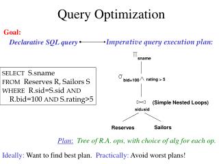
(pipeline) sname (pipeline) rating > 5 bid=100 (Block Nested loop) sid=sid Reserves Sailors Motivating Example SELECT S.sname FROM Reserves R, Sailors S WHERE R.sid=S.sid AND R.bid=100 AND S.rating>5 • Cost: 500+500*1000 I/Os • Not too bad! • Misses several opportunities: selections could have been `pushed’ earlier and no use of indexes. • Goal of optimization: Find more efficient plans that compute the same answer. Plan:
Schema for Examples Sailors (sid: integer, sname: string, rating: integer, age: real) Reserves (sid: integer, bid: integer, day: dates, rname: string) • Reserves: • Each tuple is 40 bytes long, 100 tuples per page, 1000 pages. • Assume there are 100 boats • Sailors: • Each tuple is 50 bytes long, 80 tuples per page, 500 pages. • Assume there are 10 different ratings • Assume there are 5 pages in the buffer pool!
(pipeline) sname (pipeline) bid=100 (pipeline) sname (Block Nested Loop) sid=sid (pipeline) rating > 5 bid=100 rating > 5 (pipeline) Reserves (Block Nested loop) Sailors sid=sid Reserves Sailors Alternative Plans – Push Selects 500,500 IOs 250,500 IOs
(pipeline) sname (pipeline) bid=100 (pipeline) sname (Block Nested loop) sid=sid (Block Nested loop) sid=sid rating > 5 (pipeline) Reserves bid = 100 rating > 5 Sailors (pipeline) (pipeline) Sailors Reserves Alternative Plans – Push Selects 250,500 IOs 250,500 IOs