Download
1 / 63
650 likes | 1.01k Views
Tracking. Image Processing Seminar 2008 Oren Mor. What is Tracking?. Estimating pose Possible from a variety of measured sensors Electrical Mechanical Inertial Optical Acoustic magnetic. Tracking applications - Examples. Tracking missiles Tracking heads/hands/drumsticks

E N D
Tracking Image Processing Seminar 2008 Oren Mor
What is Tracking? • Estimating pose • Possible from a variety of measured sensors • Electrical • Mechanical • Inertial • Optical • Acoustic • magnetic
Tracking applications - Examples • Tracking missiles • Tracking heads/hands/drumsticks • Extracting lip motion from video • Lots of computer vision applications • Economics • Navigation SIGGRAPH 2001
Noise • Each sensor has fundamental limitations related to the associated physical medium • Information obtained from any sensor is part of a sequence of estimates • One of the most well-known mathematical tools for stochastic estimation from noisy sensor measurement is the Kalman Filter City of Vancouver
Rudolf Emil Kalman • Born in 1930 in Hungary • BS and MS from MIT • PhD 1957 from Columbia • Filter developed in 1960-61 • Now retired SIGGRAPH 2001
What is the Kalman Filter? • Just some applied math • A linear system: f(a+b)=f(a)+f(b) • Noisy data in → hopefully less noisy out • But delay is the price for filtering… • Predictor-corrector estimator that minimizes the estimated error covariance • We’ll talk about The Discrete Kalman filter SIGGRAPH 2001
Recursive Filters • Sequential update of previous estimate • Allow on-line processing of data • Rapid adaptation to changing signals characteristics • Consists of two steps: • Prediction step: • Update step:
A The process to be estimated • Discrete time controlled process governed by linear stochastic difference equation • A is the state transition model applied to the previous state • B is the control-input model applied to the control vector • W is the process noise wikipedia
A The process to be estimated • With a measurement that is • H is the observation model, which maps the process space into the observed space wikipedia
A The process to be estimated • and are the process and measurement noise respectively • We assume • The noise vectors are assumed to be mutually independent wikipedia
Computational Origins of the filter • is the a priori state estimated at step k given knowledge of the process prior to step k • is the a posteriori state estimated at step k given measurement Kalman filter web site
Computational Origins of the filter • The a priori error estimate • The a posteriori error estimate • The a priori estimate error covariance is • The a posteriori estimate error covariance is Kalman filter web site
Computational Origins of the filter • Computing a posteriori state estimate as a linear combination • The residual reflects the discrepancy between predicted measurement and the actual measurement • K minimizes the a posteriori error covariance equation Kalman filter web site
Interesting Observations • As the measurement error covariance R approaches zero, K weights the residual is more “trusted”, is “trusted” less • As the a priori estimate error covariance approaches zero, K weights the residual less is less “trusted”, is “trusted” more Kalman filter web site
The Discrete Kalman Filter Algorithm • Time update equations are responsible for projecting forward the current state and error covariance – predictor equations • Measurement update equations are responsible for the feedback – corrector equations Kalman filter web site
Predict → Correct • Predicting the new state and its uncertainty • Correcting with the new measurement Kalman filter web site
The Discrete Kalman Filter Algorithm Kalman filter web site
Example • A truck on a straight frictionless endless road • Starts from position 0 • Has random acceleration • Measured every ∆t, imprecisely • We’ll derive a model from which we create a Kalman filter wikipedia
Example - Model • No control, so B and u is ignored • The position and velocity is described by linear state space • We assume that the acceleration ak, normally distributed, with mean 0 and STD from Newton laws of motion where wikipedia
Example - measurement • A noisy measurement of the true position. Assume the noise is normally distributed with STD where wikipedia
Example – initialization • We know the starting state with perfect percision and the covariance matrix is zero And we’re ready to run the KF iterations! wikipedia
Extended Kalman filter • Most non-trivial systems are non-linear • In the extended Kalman filter the state transition and observation model • The EKF is not an optimal estimator • If initial state or process model is wrong, the filter quickly diverges • The de facto standard in navigation systems and GPS wikipedia
Introduction • We talked about Kalman filter, which relied on a Gaussian model • Another family of algorithms uses nonparametric models • No restrictions to linear processes or Gaussian noise
Dynamic System • State transition: • State only depends on previous state • Measurement equation: • Both functions are not necessarily linear • The state noise on both equations is usually not Gaussian
Propagation in one time step Isard and Blake, IJCV
General Prediction-Update Framework • Assume that is available at time k-1 • Prediction step: (using Chapman-Kolmogoroff equation) • This is the prior to state at time k without knowing the measurement • Update step: • Compute posterior from predicted prior and new measurement
Particle Filter – general concept • If we cannot solve the integrals required for a Bayesian recursive filter analytically, we represent the posterior probabilities by a set of randomly chosen weighted samples Vampire-project
Sequential Importance Sampling • Let set of support points (samples, particles) • Whole trajectory for each particle • Let associated weights, normalized to • Then: (discrete weighted approximation to the true posterior)
Sequential Importance Sampling • Usually we cannot draw samples from directly. Assume we sample directly from a different importance function . Our approximation is still correct if • The trick: We can choose freely!
Factored sampling Isard and Blake, IJCV
Probability distribution example • Each sample is shown as a curve • Thickness proportional to the weight • Estimator of the distribution mean Movie Isard and Blake, IJCV
Sequential Importance Sampling • If the importance function is chosen to factorize such that Then one can augment old particles by to get new particles
Sequential Importance Sampling • Weight update (after some lengthly computations) • Furthermore, if (only depends on last states and observations) And we don’t need to preserve trajectories and the histories
Problem – Degeneracy problem • Problem with SIS approach: after a few iterations, most particles have negligible weight (the weight is concentrated on a few particles only) Counter measures: • Brute force: many samples • Good choice of importance density • resampling
Resampling Approaches • Whenever degeneracy rises above threshold: replace old set of samples (+weights) with new set of samples (+weights), such that sample density better reflects posterior • This eliminates particles with low weight and chooses more particles in more probable regions
Problems • Particles with high weight are selected more and more often, others die out slowly • Resampling limits the ability to parallelize the algorithm
Advantages of PF • Can deal with non-linears • Can deal with non-Gaussian noise • Can be implemented in O(Ns) • Mostly parallelizable • Easy to implement
Intoduction • Difficulties for Multiple Object Tracking • Objects may interact. • The objects may present more or less the same appearances • BraMBLe: A Bayesian Multiple-Blob Tracker, M. Isard and J. MacCormick, ICCV’01. Qi Zhao
Problem • The goal is to track an unknown number of blobs from static camera video. Qi Zhao
Number, Positions, Shapes, Velocities, … Solution • The Bayesian Multiple-BLob (BraMBLe) tracker is a Bayesian solution. • It estimates State at frame t Image Sequence Qi Zhao
Modeling idea ObservationLikelihood Posterior State Distribution Prior • Sequential Bayes ObservationLikelihood PosteriorStateDistribution Prior Instead of modeling directly, BraMBLe models and . Qi Zhao
Object State Number of objects Object Model X • The blob configuration is Qi Zhao
Object Model X Identity Velocity Shape Location Qi Zhao