Understanding Heat Diffusion: The Gaussian Distribution

1. The Heat Equation and Diffusion PHYS220 2004 by Lesa Moore DEPARTMENT OF PHYSICS Macquarie University 2004

2. Diffusion of Heat • The diffusion of heat through a material such as solid metal is governed by the heat equation. • We will not try to derive this equation. • We will compare results from the heat equation with our studies of the random walk. Macquarie University 2004

3. Initial Temperature Distribution • Consider diffusion in 1D (let a thin copper wire represent a one-dimensional lattice). • Let u(t,x) be the heat at point x at time t, with x and t integers, u(t=0,x=0)=1 and u(t=0,x)=0 if x is not zero. Macquarie University 2004

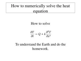
4. The Partial Differential Equation • The heat equation is a partial differential equation (PDE): • k is the diffusion coefficient. • Assume the initial distribution is a spike at x=0 and is zero elsewhere. Macquarie University 2004

5. Partial Derivatives • For functions of more than one variable, the partial derivative is the rate of change with respect to one variable with the other variable(s) fixed. • : • : • : Macquarie University 2004

6. The PDE in full • : • : • : Macquarie University 2004

7. Converting to a Difference Equation • Don’t take the limits as intervals approach zero. • Take finite time steps (Dt=1) and finite positions steps (Dx=1). Macquarie University 2004

8. Simplifying … 1 1 1 Macquarie University 2004

9. Rearranging … • Want all t+1 terms on l.h.s. and everything else on r.h.s. Macquarie University 2004

10. Modelling in Excel • Columns are x-values. • Rows are t-values. • The difference equation relates each cell to three cells in the row above. Macquarie University 2004

11. The Excel Spreadsheet • The first row (t=0) is all zeros except for the initial spike: u(t=0,x=0) = 1. • The same formula is entered in every cell from row 2 down: • A1 holds the value of k (k = 0.1) • AA3=$A$1*(Z2-2*AA2+AB2)+AA2 Macquarie University 2004

12. Filling the Spreadsheet • In Excel, it is easiest to insert the formula in the top left cell of the range, select the range and use Ctrl+R, Ctrl+D to fill the range: • -20 ≤ x ≤ 20; 0 ≤ t ≤ 60. Macquarie University 2004

13. Boundary Conditions • What happens at the boundaries? • Setting columns at x=±21 equal to zero stops the spatial evolution of the model – is this a problem? • Provided that values in neighbouring columns (x=±20) are still small at the end of the simulation, the choice of boundary conditions is not so important. • u=0 is equivalent to an absorbing boundary. Macquarie University 2004

14. Snapshots Macquarie University 2004

15. Plotting the Heat Spread Macquarie University 2004

16. Spreadsheet Results • Conservation of heat can be demonstrated by adding the values in a row (a row is a time step). • Values in a row should add to 1. • Checking the sum in a row is good test of numerical accuracy. • Heat diffusion looks like a Gaussian distribution. Macquarie University 2004

17. The Distribution • The simulation satisfies conservation of energy (total heat along a row = 1). • Does the Gaussian distribution satisfy this condition too (area under curve = 1)? • The initial spike can be thought of as a very sharp, very narrow Gaussian. • For t>0, need to integrate the Gaussian. • “Normalised” if integral yields unity. Macquarie University 2004

18. Normalisation of the Gaussian • Formula for Gaussian with m = 0. • Use a trick for the integral: Macquarie University 2004

19. The integral becomes Macquarie University 2004

20. But using and Macquarie University 2004

21. Cancelling Macquarie University 2004

22. Then use the substitution: Macquarie University 2004

23. And finally: Macquarie University 2004

24. The integral proves that the Gaussian is normalised to unity – the area under the curve is one. • But the heat equation is a function of x and t, and uses a constant k. • k and t must be included in the s term of the Gaussian if we are to say our model satisfies this distribution. Macquarie University 2004

25. What is s ? • From the Random Walk, we learned that s√t. • Try a guess: • The Gaussian becomes: Macquarie University 2004

26. Derivatives of the Gaussian • Space derivatives: • The time derivative is left as an exercise … Macquarie University 2004

27. The Gaussian satisfies the Heat Equation • It can be shown that the heat equation is satisfied by our guess. • The distribution integrates to unity (conservation of energy). • The spread of heat is given by s of the Gaussian (normal) distribution. Macquarie University 2004

28. Diffusion and the Random Walk • The initial temperature spike grows into a Gaussian distribution according to the 1D heat equation. • The width s grows in proportion to the square root of elapsed time. • Heat and diffusion can be understood in terms of the “random walk”. Macquarie University 2004

29. Other Conditions • The initial condition may not be a spike, but could be some initial distribution: u(x,0)=g(x). • The boundary conditions may not be absorbing, but could be continuous. • The thermal diffusivity constant k may not be constant, but may vary with x or t. Macquarie University 2004

30. Summary • The heat equation is a PDE. • By separating space and time variables, we see that a Gaussian that spreads as √t is a solution. • We can model the differential equation as a difference equation in Excel and see the same effect. • The spread of heat is a physical example of a random walk. Macquarie University 2004

31. Acknowledgements • This presentation was based on lecture material for PHYS220 presented by Prof. Barry Sanders, 2000-2003. • Additional Reference: • Folland, Fourier Analysis and its Applications, 1992. Macquarie University 2004