Download

1 / 42
420 likes | 640 Views
Exam 4 – Optional Times for Final Two options for completing Exam 4 Thursday (4/25/13) Tuesday (4/30/13) Must sign up to take Exam 4 on Tuesday (4/23) Only need to take one exam – these are two optional times. Sign up today to take Exam 4 at later date: April 30 th.

E N D
Exam 4 – Optional Times for Final • Two options for completing Exam 4 • Thursday (4/25/13) • Tuesday (4/30/13) • Must sign up to take Exam 4 on Tuesday (4/23) • Only need to take one exam – these are two optional times Sign up today to take Exam 4 at later date: April 30th No need to sign up if you are taking it at regular time (April 25th)
MGMT 276: Statistical Inference in ManagementSpring, 2013 Welcome
Statistical Inference in Management Instructor:Suzanne Delaney, Ph.D. Office:405 “N” McClelland Hall Phone:621-2045 Email:delaney@u.arizona.edu Office hours:2:00 – 3:30Mondays and Fridays and by appointment
Readings for Exam 4 Lind Chapter 13: Linear Regression and Correlation Chapter 14: Multiple Regression Chapter 15: Chi-Square Plous Chapter 17: Social Influences Chapter 18: Group Judgments and Decisions Study Guide online (shorter and longer version)
Use this as your study guide Over next couple of lectures 4/23/13 • Multiple Regression Review • Exam 4 Review • Teacher Evaluations
+0.85 This appears to be a strong positive relationship 3
+0.9199 3 .878 yes yes The relationship between the hours worked and weekly pay is a strong positive correlation. This correlation is significant, r(3) = 0.92; p < 0.05 positive strong up down 55.286 6.0857 y' = 6.0857x + 55.286 207.43 85.71 .846231 or 84% 84% of the total variance of “weekly pay” is accounted for by “hours worked” For each additional hour worked, weekly pay will increase by $6.09
400 380 360 Wait Time 340 320 300 280 7 8 6 5 4 Number of Operators
-.8 The relationship between wait time and number of operators working is negative and strong. 3 -.73 3 .878 No No The relationship between wait time and number of operators working is negative and strong, but not reliable enough to reach significance. This correlation is not significant, r(3) = -0.73; n.s. negative strong number of operators working goes up, wait time goes down 458 -18.5 y' = -18.5x + 458 384 seconds 310 seconds .53695 or 54% The proportion of total variance of wait time accounted for by number of operators is 54%. For each additional operator added, wait time will decrease by 18.5 seconds
10 Amount spent on snacks 8 6 4 2 20 10 40 30 50 Age of movie goers
-.292 8 .632 No No The relationship between age of movie goers and the amount spent on snacks is negative and weak. This correlation is not significant, r(8) = -0.29; n.s. negative weak the age of the movie goes up spending goes down 6.96 -.053 y' = 6.96 - .053x $5.635 $4.575 .085264 or 8.5% The proportion of total variance of amount of money spent that is accounted for by age of the movie goer is 8.5% For each additional year older the movie goer is, we expect they will spend 5.3 cents less on snacks
7 6 Shipping Cost (000) 5 4 3 2 800 600 1200 1000 Number of Orders
.8196 10 .576 Yes Yes The relationship between the number of orders and shipping costs is positive and strong. This correlation is significant, r(10) = 0.82; p < 0.05 positive strong orders increase, shipping costs will go up – 31.19 4.9322 y' = 4.9322x – 31.19 $4,901.01 $3,421.35 .6717 or 67.17% The proportion of total variance of shipping cost that is accounted for by number of orders is 67.17% For each unit increase in orders, shipping cost will go up by $4.93
500 400 300 200 100 500 400 300 200 100 500 400 300 200 100 Heating Cost Heating Cost Heating Cost 0 20 40 60 80 0 20 40 60 80 0 20 40 60 80 Average Temperature Insulation Age of Furnace r(18) = - 0.50 r(18) = - 0.40 r(18) = + 0.60 r(18) = - 0.811508835 r(18) = - 0.257101335 r(18) = + 0.536727562
500 400 300 200 100 500 400 300 200 100 500 400 300 200 100 Heating Cost Heating Cost Heating Cost 0 20 40 60 80 0 20 40 60 80 0 20 40 60 80 Average Temperature Insulation Age of Furnace r(18) = - 0.50 r(18) = - 0.40 r(18) = + 0.60 r(18) = - 0.811508835 r(18) = - 0.257101335 r(18) = + 0.536727562
+ 427.19 - 4.5827 -14.8308 + 6.1010 - 4.5827 x1 - 14.8308 x2 427.19 + 6.1010 x3 Y’ =
+ 427.19 - 4.5827 -14.8308 + 6.1010 - 4.5827 x1 - 14.8308 x2 427.19 + 6.1010 x3 Y’ =
+ 427.19 - 4.5827 -14.8308 + 6.1010 - 4.5827 x1 - 14.8308 x2 427.19 + 6.1010 x3 Y’ =
+ 427.19 - 4.5827 -14.8308 + 6.1010 - 4.5827 x1 - 14.8308 x2 427.19 + 6.1010 x3 Y’ =
+ 427.19 - 4.5827 -14.8308 + 6.1010 - 4.5827 x1 - 14.8308 x2 427.19 + 6.1010 x3 Y’ =
4.58 14.83 6.10 - 4.5827(30) +6.1010 (10) -14.8308 (5) 427.19 Y’ = + 61.010 - 74.154 - 137.481 = $ 276.56 = $ 276.56 427.19 Y’ = Calculate the predicted heating cost using the new value for the age of the furnace Use the regression coefficient for the furnace ($6.10), to estimate the change
4.58 14.83 6.10 - 4.5827(30) +6.1010 (10) -14.8308 (5) 427.19 Y’ = + 61.010 - 74.154 - 137.481 = $ 276.56 427.19 Y’ = - 4.5827(30) +6.1010 (10) -14.8308 (5) 427.19 Y’ = These differ by only one year but heating cost changed by $6.10 282.66 – 276.56 = 6.10 + 61.010 - 74.154 - 137.481 = $ 276.56 = $ 276.56 427.19 Y’ = $ 276.56 - 4.5827(30) +6.1010 (11) -14.8308 (5) 427.19 Y’ = + 67.111 - 74.154 - 137.481 = $ 282.66 427.19 Y’ = Calculate the predicted heating cost using the new value for the age of the furnace Use the regression coefficient for the furnace ($6.10), to estimate the change
4.0 3.0 2.0 1.0 4.0 3.0 2.0 1.0 4.0 3.0 2.0 1.0 GPA GPA GPA 0 200 300 400 500 600 0 1 2 3 4 0 200 300 400 500 600 High School GPA SAT (Verbal) SAT (Mathematical) r(7) = 0.50 r(7) = + 0.80 r(7) = + 0.80 r(7) = + 0.911444123 r(7) = + 0.616334867 r(7) = + 0.487295007
4.0 3.0 2.0 1.0 4.0 3.0 2.0 1.0 4.0 3.0 2.0 1.0 GPA GPA GPA 0 200 300 400 500 600 0 1 2 3 4 0 200 300 400 500 600 High School GPA SAT (Verbal) SAT (Mathematical) r(7) = 0.50 r(7) = + 0.80 r(7) = + 0.80 r(7) = + 0.911444123 r(7) = + 0.616334867 r(7) = + 0.487295007
4.0 3.0 2.0 1.0 4.0 3.0 2.0 1.0 4.0 3.0 2.0 1.0 GPA GPA GPA 0 200 300 400 500 600 0 1 2 3 4 0 200 300 400 500 600 High School GPA SAT (Verbal) SAT (Mathematical) r(7) = 0.50 r(7) = + 0.80 r(7) = + 0.80 r(7) = + 0.911444123 r(7) = + 0.616334867 r(7) = + 0.487295007
4.0 3.0 2.0 1.0 4.0 3.0 2.0 1.0 4.0 3.0 2.0 1.0 GPA GPA GPA 0 200 300 400 500 600 0 1 2 3 4 0 200 300 400 500 600 High School GPA SAT (Verbal) SAT (Mathematical) r(7) = 0.50 r(7) = + 0.80 r(7) = + 0.80 r(7) = + 0.911444123 r(7) = + 0.616334867 r(7) = + 0.487295007
No - 0 .41107
No - 0 .41107 Yes + 1.2013
No - 0 .41107 Yes + 1.2013 No 0.0016
No - 0 .41107 Yes + 1.2013 No 0.0016 No - 0 .0019
No - 0 .41107 Yes + 1.2013 No 0.0016 No - 0 .0019 High School GPA
No - 0 .41107 Yes + 1.2013 No 0.0016 No - 0 .0019 High School GPA + 1.2013x1 + 0 .0016 x2 Y’ = - 0 .41107 - 0 .0019 x3
1.201 .0016 .0019 + 1.2013x1 + 0 .0016 x2 Y’ = - 0 .41107 - 0 .0019 x3 + 1.2013(2.8) = 2.76 2.76 + 0.0016 (430) Y’ = - 0 .411 - 0 .0019 (460)
1.201 .0016 .0019 + 1.2013x1 + 0 .0016 x2 Y’ = - 0 .41107 - 0 .0019 x3 + 1.2013(3.8) = 3.96 3.96 + 0 .0016 (430) Y’ = - 0 .411 - 0 .0019 (460)
1.201 .0016 .0019 2.76 3.96 = 1.8016 3.96 - 2.76 = 1.2 Yes, use the regression coefficient for the HS GPA (1.2), to estimate the change
Please hand in your homework
Homework: No more homework!! Please click in My last name starts with a letter somewhere between A. A – D B. E – L C. M – R D. S – Z
Today we will be reviewing for the test using clicker questions. Please note these will not appear on the class website Review Exam 4
Thank you! See you next time!!