Download
1 / 19
200 likes | 511 Views
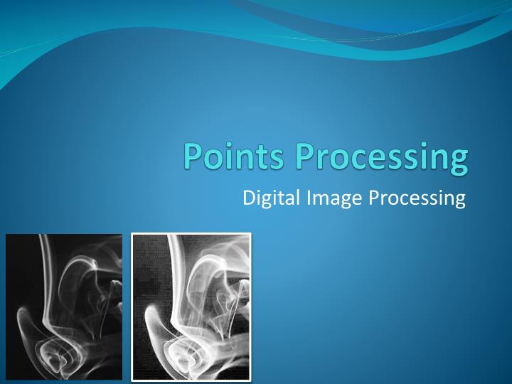
Points Processing. Digital Image Processing. Introduction. Any image-processing operation transforms the gray values of the pixels. Image-processing operations may be divided into three classes: Transforms Neighborhood processing Point operations. Neighborhood processing

E N D
Points Processing Digital Image Processing
Introduction • Any image-processing operation transforms the gray values of the pixels. • Image-processing operations may be divided into three classes: • Transforms • Neighborhood processing • Point operations Neighborhood processing Point operations Ch4-p.65
Arithmetic Operations: Complement • The complement of a gray-scale imageis its photographic negative • type double (0.0~1.0) • 1-m • type uint8 (0~255) • 255-m
Histogram • A graph indicating the number of times each gray level occurs in the image
Histogram Stretching • A table of the numbers ni of gray values • We can stretch out the gray levels in the center of the range by applying the piecewise linear function Stretch function Original histogram
Histogram Stretching: imadjust • imadjust is designed to work equally well on images of type double, uint8, or uint16 • the values of a, b, c, and d must be between 0 and 1 • the function automatically converts the image im (if needed) to be of type double • Note that imadjust does not work exactly the same way of the stretching function as shown in previous slide
Histogram Stretching: imadjust • The imadjust function has one other optional parameter: the gamma value >> img = imread('pollen.tif'); >> m_ad= imadjust(img,[],[],2); >> figure, imshow(m_ad);
Histogram Stretching: histpwl >> img = imread('tire.tif'); >> a = [0 .25 .5 .75 1]; >> b = [0 .75 .25 .5 1]; >> pwl = histpwl(img,a,b); >> figure, imshow(pwl); >> figure, plot(img,pwl,'.') Piece-wise linear stretching
Histogram Equalization • An entirely automatic procedure • Suppose our image has L different gray levels, 0, 1, 2, . . . , L − 1, and gray level i occurs nitimes in the image wheren=n0 +n1 +n2 +· · ·+nL−1
Histogram Equalization: Example • Suppose a 4-bit gray-scale image has the histogram shown below, associated with a table of the numbers ni of gray values (L-1)/n
Histogram Equalization: Example >> p = imread('pout.tif'); >> figure, imshow(p), figure, imhist(p), axis tight; >> ph = histeq(p); >> figure, imshow(ph), figure, imhist(ph), axis tight;
Histogram Equalization: Appendix • WHY IT WORKS ? • If we were to treat the image as a continuous function f (x, y)and the histogram as the area between different contours, then we can treat the histogram as a probability density function.
Lookup Table • Point operations can be performed very effectively by using a lookup table, known more simply as an LUT • e.g., the LUTcorresponding to division by 2 looks like >> b = imread('blocks.tif'); >> T = uint8(floor([0:255]/2)); >> >> % blocks image serves as LUT >> % LUT indices must be positive >> % integers or logicals >> b2 = T(b+1); >> figure, imshow(b); >> figure, imshow(b2);
Lookup Table vs. Histogram Stretching • As another example, suppose we wish to apply an LUT to implement the contrast-stretching function t1 = 0.667*[0:96]; t2 = 2*[97:160]-128; t3 = 0.6632*[161:255]+85.8947; T = uint8(floor([t1 t2 t3])); b = imread('pollen.tif'); b2 = T(b+1); figure, imshow(b), figure, imhist(b), axis tight; figure, imshow(b2), figure, imhist(b2), axis tight; figure, plot(T), axis tight;