Download
1 / 66
660 likes | 846 Views
Computational Transportation Science. Ouri Wolfson Computer Science. Vision. Take advantage of advances in Wireless communication (communicate) Mobile/static Sensor technologies (integrate) Geospatial-temporal information management (analyze) To address transportation problems Congestion

E N D
Computational Transportation Science Ouri Wolfson Computer Science
Vision • Take advantage of advances in • Wireless communication (communicate) • Mobile/static Sensor technologies (integrate) • Geospatial-temporal information management (analyze) • To address transportation problems • Congestion • Safety • Mobility • Energy • Environmental
Funded by the National Science Foundation ($3M+) Train about 20 Scientists Will develop novel classes of applications Colleges: engineering, business, urban planning $30K/year stipend, international internships IGERT Ph.D. program in Computational Transportation Science Transportation Information Technology
Outline • Abstraction of concepts from sensor data: extracting semantic locations from GPS traces. • Coping with imprecision and uncertainty: map matching. • Mixed environments: information in vehicular and other peer-to-peer networks. • Managing spatial-temporal data: compression. • Software tools: Databases with • spatial, • temporal, • uncertainty capabilities for • Tracking, • analysis, • routing;
Introduction – location information • Location information • Physical location • Provided by positioning systems • GPS: (122.39, 239.11, 11:20am) • Unreadable by users • Semantic location • Not directly provided by positioning systems • Dominick’s grocery store, 1340 S. Canal St. • Dermatologist’s office • Home • Useful to users
Introduction – problem statement • Physical location -> semantic location • Devices • Outdoor positioning systems • Internet access • Application examples: • context awareness of mobile devices (autocomplete) • Reminder applications • “Total Recall” by Gordon Bell
Main Input and Output • Input: Trajectory: T =(x1, y1, t1), (x2, y2, t2), …, (xn, yn, tn) • Output 1: Semantic location • Location name (BestBuy) • Semantic category • Business type (electronics store), • office • home • Street address • Output 2: Semantic location log file • (date, begin_time, end_time, semantic location)
Online and offline versions • Online: determine the current location • On mobile device • Based on incomplete trip trajectory • Offline: Determine multiple past locations • Based on complete trip trajectory
Auxiliary inputs • Profile • Calendar – (event date, semantic location) • Address Book – (phone number, semantic location) • Phone Call List – (calling date, semantic location) • Web Page List - (visiting date, semantic location) • Destination List – (searching date, address) • User’s Feedback • Confirmed list • Denied list
Step1 - Stay extraction • Stay • Loss of GPS signal • To spend at least min_time in an area with the diameter no larger than d. • (stay_position, date, stay_start, stay_end) Juhong Liu, Ouri Wolfson, Huabei Yin, UIC
Step2 – Street address candidates • Reverse Geocoding • Physical location (stay_position) -> street address • Traditional geocoding method • Nearest street address • Incorrect result Street address candidates: the street addresses within k meters (graph distance) from stay_position. Juhong Liu, Ouri Wolfson, Huabei Yin, UIC
Step3-semantic location candidates • Street address candidates -> semantic location candidates • Yellow pages • Such as switchboard.com • Profile • Calendar, Address Book, Phone Call List, Web Page List, Destination List, User's Feedback
At end of step 3: A set of Semantic Location candidates • Semantic location • Location name (BestBuy) • Semantic category • Business type (electronics store; theater), • office • home • Street address
Step4- three utilities calculation • For each semantic location SL in set of candidates compute: • Semantic category (SC) utility: likelihood of semantic category, given semantic log (history) • Street address (SA) utility: likelihood the street address, given the stay location • Profile (P) utility: Likelihood of SL, given profile P
Outline • Abstraction of concepts from sensor data: extracting semantic locations from GPS traces. • Coping with imprecision and uncertainty: map matching. • Mixed environments: information in vehicular and other peer-to-peer networks. • Spatial-temporal data: compression. • Software tools: Databases with • spatial, • temporal, • uncertainty capabilities for • Tracking, • analysis, • routing;
Problem • Most information systems are client/server • Nearby mobile devices are inaccessible • Parking slot info • Video of road construction • Malfunctioning brakelight • Taxi cab • Ride-share opportunity
resource 8 resource-query C resource-query A resource 1 resource 2 resource 3 resource-query B resource 4 resource 5 Environment Pda’s, cell-phones, sensors, hotspots, vehicles, with short-range wireless A central server does not necessarily exist Short-range wireless networks wi-fi (100-200 meters) bluetooth (2-10, popular) zigbee Unlicensed spectrum (free) High bandwidth Bandwidth-Power/search tradeoff Local query Local database “Floating database” Resources of interest in a limited geographic area possibly for short time duration Applications coexist
Mobile Local Search: applications • social networking (wearable website) • Personal profile of interest at a convention • Singles matchmaking • Games • Reminder • mobile advertising (coupons, rfid-tag info) • Sale on an item of interest at mall • Music-file exchange • Transportation • emergency response • Search for victims in a rubble • military • Sighting of insurgent in downtown Mosul in last hour • asset management and tracking • Sensors on containers exchange security information => remote checkpoints • mobile collaborative work • tourist and location-based-services • Closest ATM
How to enable Mobile P2P applications? • Develop a platform for building them
Problems in data management • Query processing • Dissemination analysis • Participation incentives
Floating (Probe) car data • Periodically the ITA on a vehicle generates • a velocity report: • Vehicle id IL391645 • Average speed 45mph • Time 3:49:45pm • Location (12345.25, 4321.52) • Travel direction east ・・・ A Segment of the road network
P2P method Each vehicle communicates reports to other vehicles using short-range (e.g. 300 meters), unlicensed, wireless spectrum, e.g. 802.11
Multimedia info: view/hear traffic conditions 1 mile ahead by a click on your smartphone.
Query Processing Strategies WiMaC paradigm: WiFi-disseminate, Match Wifi/cellular-respond media media Q Z M-producer Q-producer (a) media and Q are initially disseminated. They collocate at Z. Q Z M-producer Q-producer (b) Z sends Q to M-producer via cellular media Z M-producer Q-producer (c) M-producer sends media to Q-producer via cellular WiMaC Design Space • Evaluation criteria: • Throughput • Response time • Wi-Fi communication volume • Cellular communication volume
Comparison Results 7b (media,meta,query)-cell 6b (media,query)-cell WiFi-cellular strategies 1 (media) push - media 4b (media,meta)-cell 2b (meta)-cell pull 3a (query)-WiFi 7b (media,meta,query)-cell hy - MuM - cell 5b (media,query)-cell 3b (query)-cell hy 6b (meta,query)-cell - meta - cell 1 (media) 3a (query)-WiFi WiFi-only strategies 5a (media,query)-WiFi 2a (meta)-WiFi 4a (media,meta)-WiFi 6a (meta,query)-WiFi 7a (media,meta,query)-WiFi X Y: Strategy X dominates strategy Y X Y: Strategy X weakly dominates strategy Y simulations dominance analysis
Outline • Abstraction of concepts from sensor data: extracting semantic locations from GPS traces. • Coping with imprecision and uncertainty: map matching. • Mixed environments: information in vehicular and other peer-to-peer networks. • Spatial-temporal data: compression • Software tools: Databases with • spatial, • temporal, • uncertainty capabilities for • Tracking, • analysis, • routing;
Data Compression -- Motivation • Tracking the movements of all vehicles in the USA needs approximately 4TB/day (GPS receivers sample a point every two seconds).
Trajectory Lossy-Compression • approximate a trajectory by another which is not farther than ε. e e
Desiderata for Trajectory Compression • bounded error when answering queries on compressed trajectories.
Relational-Oriented Queries • Point queries: • Where (T,t): where is the moving object with trajectory T at time t • When (T,x,y): when is the moving object with trajectory T at location (x,y) • Range queries (R,t1,t2,O): retrieve the moving objects (i.e. trajectories) of O that are in region R between times t1 and t2. • Nearest neighbor (t,T,O): retrieve the object of O that is closest to trajectory T at time t • Join queries (O,d): Retrieve the pairs of objects of O that are within distance d.
Distance Functions • The distance functions considered are: • E3: 3D Euclidean distance. • E2: Euclidean distance on 2D projection of a trajectory • Eu: the Euclidean distance of two trajectory points with same time. • Et: It is the time distance of two trajectory points with same location or closest Euclidean distance. • #(T'2) ≤ #(T'3) ≤ #(T'u), which is also verified by experimental saving comparison.
Soundness of Distance Functions • Soundness: bound on the error when answering spatio-temporal queries on compressed trajectories. • The appropriate distance function depends on the type of queries expected on the database of compressed trajectories. • If all spatio-temporal queries are expected, then Eu and Et should be used. • If only where_at, intersect, and nearest_neighbor queries are expected, then the Eu distance should be used.
Aging of Trajectories • Increase the tolerance ε as time progresses • Aging friendliness property: If ε1ε2 then T’ =Comp(Comp(T, ε1 ), ε2) = Comp(T, ε2) (associative) Theorem: The DP algorithm is aging-friendly, whereas the optimal algorithm is not.
Outline Abstraction of concepts from sensor data: extracting semantic locations from GPS traces. Coping with imprecision and uncertainty: map matching. Mixed environments: information in vehicular and other peer-to-peer networks. Spatial-temporal data: compression. Software tools: Databases with spatial, temporal, uncertainty capabilities for Tracking, analysis, routing;
Matching Methods ---- Straightforward Snapping • A, B: road segments • a, b: GPS points • A, B: road segments • a, b: GPS points
Weight-based Matching • Compute the weight of each road segment (block) • Compute the shortest weight path between the start and the end GPS points as the route of the moving object
Matching Variants Offline Find the overall route of a vehicle after the trip is over Online Snapping Real time, i.e. every 2 minutes (online frequency) Determine the road segment on which the vehicle is currently located
Experiments ---- Offline Evaluation method Edit Distance The smallest number of insertions, deletions, and substitutions required to change the snapped route to the correct route Correct matching percentage (OFFcorrect) OFFcorrect = 100(1 – ed/n)
Results On average, weight-based alg. is correct up to 94% of the time, depending on the GPS sampling interval. It is always superior to the straightforward closest-block snapping. Correct matching decreases significantly when GPS sampling intervals are larger than 120 seconds
Outline • Abstraction of concepts from sensor data: extracting semantic locations from GPS traces. • Coping with imprecision and uncertainty: map matching. • Mixed environments: information in vehicular and other peer-to-peer networks. • Spatial-temporal data: compression. • Software tools: Databases with • spatial, • temporal, • uncertainty capabilities for • Tracking, • analysis, • routing;
Basic element of a moving objects database: a trajectory Time 3d-TRAJECTORY Present time X 2d-ROUTE Y Future Trajectory: Motion plan Past trajectory: GPS trace
Why are traditional databases inappropriate to manage trajectories? 11 R sometime always 10 10 11 Retrieve the objects that are in R sometime/always between 10 and 11am SELECT o FROM MOVING-OBJECTS WHERE Sometime/Always(10,11) inside (o, R)
Why are traditional databases inappropriate to manage trajectories? • Discrete vs. Continuous data • Operators of the language that are natural in the domain • Uncertainty
Uncertainty operators in spatial range queries possibly and definitely semantics based on branching time SELECT o FROM MOVING-OBJECTS WHEREPossibly/Definitely Inside (o, R) R definitely possibly uncertainty interval
Possible Motion Curve (PMC) and Trajectory Volume (TV) • PMC is a continuous function from Time to 2D • TV is the boundary of the set of all the PMCs (resembles a slanted cylinder)
Predicates in spatial range queries Possibly – there exists a possible motion curve Definitely -- for all possible motion curves • possibly-sometime = sometime-possibly • possibly-always • always-possibly • definitely-always = always-definitely • definitely-sometime • sometime-definitely
probability density function database location Uncertainty interval Uncertainty in Language - Quantitative Approach