Download
1 / 29
310 likes | 544 Views
Exact and Efficient Construction of Planar Minkowski Sums Using the Convolution Method. Ron Wein. 14 th ESA Zuirch, July 2006. Computing Minkowski Sums. . =. Planar Minkowski Sums. Given two sets A and B in the plane, their Minkowski sum, denoted A B , is:

E N D
Exact and Efficient Construction of Planar Minkowski Sums Using the Convolution Method Ron Wein 14th ESA Zuirch, July 2006
= Planar Minkowski Sums • Given two sets A and B in the plane, their Minkowski sum, denoted AB, is: • A B = {a + b | a A, b B}
The Sum Complexity (I) • We are given two polygons P and Q with mandn vertices respectively. If both polygons are convex, the complexity of their sum is m + n, and we can compute it in (m + n) time using a very simple procedure.
The Sum Complexity (II) • If only one of the polygons is convex, the complexity of their sum is (mn). • If both polygons are non-convex, the complexity of their sumis (m2n2).
Q1 P1 Q P2 P Q2 PQ The Decomposition Method • The prevailing method for computing the sum of two non-convex polygons: Decompose P and Q into convex sub-polygons, compute the pair-wise sums of the sub-polygons and obtain the union of these sums.
Computing the Union • Given a set of polygons P1, …, Pk with counterclockwise (positive) orientation, construct the arrangement of their edges. • Set N(fu) = 0 for the unbounded face fu. Then compute N(f ) for each other face using a simple BFS traversal. • All faces with N(f ) > 0 contribute to the union. (1) (2) (0) (0) (1) (1) (2)
t s T S Convolution of Planar Tracings(Guibas, Ramshaw and Stolfi, 1983) • A planar tracingT comprises a continuous set of points. Each point t T is associated with a direction dir(t). • The convolution of two planar tracings S and T, denoted S T, comprises the pair-wise sum of all points s S and t T such that dir(s) = dir(t).
P dir(p) Q p Convolution of Polygons (I) • A polygonal tracingP consists of moves (going along an edge in a fixed direction), and turns (rotating at a vertex). • For a vertex p of P, dir(p) is a continuous range of directions. The convolution P Q therefore contains the sum of each edge of the polygonal tracing Q, whose direction is in dir(p), with p.
(0) (0) (1) (2) Convolution of Polygons (II) • At the worst case, the convolution of two polygons P Q consists of (mn) line segments. • Guibas and Seidel (1987) gave an output-sensitive algorithm for computing the convolution segments in O(m + n + K) time. • The convolution segments form closed cycles. The Minkowski sum P Q contains all points whose winding number with respect to any of the convolution cycles is positive.
PQ The Case of a Single Cycle Q P 2 0 0 2 2 1
The Case of Multiple Cycles • We compute the first cycle, starting from the two bottommost vertices in P and Q. • If P or Q are convex, we are done.Otherwise, while it is possible to locate two vertices pP andqQ that should be in the convolution, construct an additional convolution cycle.
About CGAL • CGAL is a collaborative effort of several sites in Europe and Israel, a C++ library providing useful and reliable geometric algorithms. • Participating cites: • Utrecht University, The Netherlands • Tel-Aviv University, Israel • INRIA Sophia-Antipolis, France • ETH Zürich, Switzerland • MPII Saarbrücken, Germany • Freie Universität Berlin, Germany
The CGAL Arrangement Package • Supports the construction of maintenance of 2D arrangements – planar subdivisions induced by a set of planes. • Handles a variety of curves. Each family of curves (line segments, polylines, circular arcs, conic arcs, etc.) is handled by a geometric traits-class. • Handles degenerate cases robustly and accurately, using the exact computation paradigm. Tangencypoints Common intersectionpoints
Implemented in thePartition_2 package • Available decomposition methods: • Optimal. • Hertel-Mehlhorn’s approximation scheme. • Greene’s approximation scheme. • The small-side angle-bisector approximation scheme. The Decomposition Method • The Minkowski-sum package re-implements the robust algorithms for sum-computations using the convex polygon-decomposition method (Agarwal, Flato and Halperin, 2000).
The Convolution Method • The first software that robustly implements the convolution algorithms for polygons. • Uses the same infrastructure for multi-way polygon union, used by the decomposition method. The same algorithm also works for the case of closed convolution cycles.
Low-Dimensional Features • The Minkowski sum of two polygons may contain low-dimensional features (isolated vertices and antennas). • The package can treat themas follows: • discard them (output theregularized sum), or • give access to themthrough the underlyingarrangement.
Experimental Input Sets (I) stars chain fork comb
Experimental Input Sets (II) cavity random knife country
PBr Polygon Offsetting using the Convolution Method Br P 2 Computing the convolution cycle … Computing the induced arrangement and the winding numbers … 0 0 2 2 1
q2 q1 Offsetting a Polygon Edge (I) = - 90º p2 = (x2, y2) p1 = (x1, y1)
Solution no. 1: Represent the offset edge as a segments of a (degenerate) conic curve with rational coefficients: Offsetting a Polygon Edge (II) • If the line supporting p1p2 is ax + by + c = 0,then the line supporting q1q2 is ax + by + (c + ℓr) = 0. • Problem: In the general case, offset arcs are not supported by rational lines!
1. Find ’1 and ’2 such that sin(’j), cos(’j) are rational. 2. Compute q’j = (xj + rcos(’j), yj + rsin(’j)). 3. Compute the intersection q’ of the two tangents at q’1 and q’2. Use the polyline q’1q’q’2 as an approximation. q’2 q’ q’1 ’2 ’1 Our Approximation Scheme p2 p1
Running Times ❶ ❶ ❷ ❷ ❸ ❹ ❺ ❸ ❹ (Pentium IV 3 GHz, in milliseconds) ❺