Download
1 / 18
200 likes | 597 Views
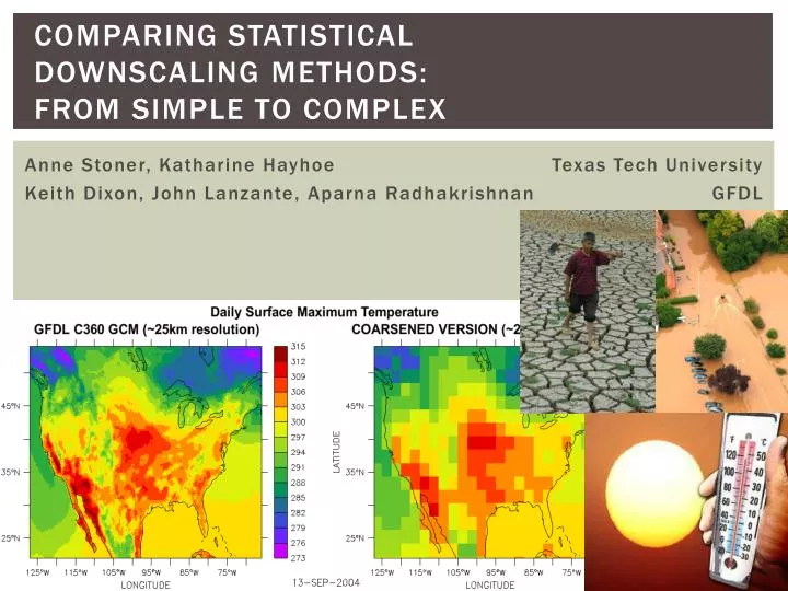
Comparing statistical downscaling methods: From simple to complex. Anne Stoner, Katharine Hayhoe Texas Tech University Keith Dixon, John Lanzante , Aparna Radhakrishnan GFDL. approach. Goal: Evaluate and compare multiple statistical downscaling methods using the same framework

E N D
Comparing statistical downscaling methods: From simple to complex Anne Stoner, Katharine Hayhoe Texas Tech University Keith Dixon, John Lanzante, AparnaRadhakrishnan GFDL
approach • Goal: Evaluate and compare multiple statistical downscaling methods using the same framework • Monthly and daily versions of Delta, Quantile Mapping, and Asynchronous Regional Regression Model • Variables – • Minimum, maximum daily 2m temperature • Daily accumulative precipitation • Input: GFDL-HiRES experimental model as both model and observations • OBS: 25km GFDL-HiRES (1979-2008) • Model: 200km coarsened GFDL-HiRES (1979-2008, 2086-2095) • Output: Daily 25km downscaled Tmin, Tmax, Prcp (2086-2095)
Method 1: Delta Change • Calculates average difference between present and future GCM simulations, then adds that difference to the observed time series for the point of interest • Here: individually for each high-resolution grid cell • Assumptions – • GCMs are more successful at simulating changes in climate rather than actual local values • Stationarity in local climate variability
Method 2: quantile mapping (e.g.bcsd) • Projects PDFs for monthly or daily simulated GCM variables onto historical observations • Changes the shape of the simulated PDF to appear more like the observed PDF, but allowing the mean and variance of the GCM to change in accordance with GCM future simulations
Method 3: quantile regression (e.g. ARRM) • Asynchronous Regional Regression Model • Daily quantile regression using piecewise linear segments to improve fit for the training period • Individual monthly models allows for different distributions throughout the year
Colorado National Monument, CO Delta Comparison • The shape of the resulting downscaled distribution depends highly on the downscaling method used Quantile Mapping ARRM
conclusions • Comparing multiple downscaling methods in a standardized framework gives us useful information • If someone has already used a certain downscaling method they can correctly interpret the biases • If someone is trying to decide which method to use, this can help their decision, because there’s no perfect method • Simple methods can be fine for studying monthly/annual means, daily output for low latitudes • More complex methods are required when studying climate extremes and high latitudes
Next steps • Downscale relative humidity • Figure out physical causes of the biases we’re seeing • Explore the influence of different predictors • Incorporate more downscaling techniques