Download
1 / 144
1.44k likes | 1.46k Views
Explore cost considerations, ordering systems, and models for efficient inventory management. Learn about ordering policies, economic order quantity models, and quantity discounts. Optimize batch sizes and understand stock levels in single-echelon systems.

E N D
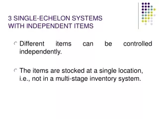
3 SINGLE-ECHELON SYSTEMS WITH INDEPENDENT ITEMS • Different items can be controlled independently. • The items are stocked at a single location, i.e., not in a multi-stage inventory system.
3.1 Costs • Holding costs - Opportunity cost for capital tied up in inventory - Material handling costs -Costs for storage - Costs for damage and obsolescence - Insurance costs - Taxes
Ordering or Setup Costs - setup and learning - administrative costs associated with the handling of orders - transportation and material handling.
Shortage Costs or Service Constraints - extra costs for administration - price discounts for late deliveries - material handling and transportation. • If the sale is lost, the contribution of the sale is also lost. In any case it usually means a loss of goodwill. - component missing - rescheduling, etc. • Because shortage costs are so difficult to estimate, it is very common to replace them by a suitable service constraint.
3.2 Different Ordering Systems • 3.2.1 Inventory position • Inventory position = stock on hand + outstanding orders - backorders. • Inventory level = stock on hand - backorders.
3.2.2 Continuous or Periodic Review • As soon as the inventory position is sufficiently low, an order is triggered. We denote this continuous review. • L = lead-time. • T = review period, i. e., the time interval between reviews.
Inventory position R+Q R Inventory level L L 3.2.3 Different Prdering Policies • (R, Q) policy • Figure 3.1 (R, Q) policy with continuous review. Continuous demand.
(R, Q) Policy • When the inventory position declines to or below the reorder point R, a batch quantity of size Q is ordered. (If the inventory position is sufficiently low it may be necessary to order more than one batch to get above R) .
Inventory position Inventory level Time L L • (s, S) Policy Figure 3.2 (s, S) policy, periodic review. • When the inventory position declines to or below s, we order up to the maximum level S.
3.3.1 Classical Economic Order Quantity Model • Harris (1913), Wilson (1934), Erlenkotter (1989) - Demand is constant and continuous. - Ordering and holding costs are constant over time. - The batch quantity does not need to be an integer. - The whole batch quantity is delivered at the same time. - No shortages are allowed.
Notation: H = holding cost per unit and time unit A = ordering or setup cost D = demand per time unit Q = batch quantity C = costs per time unit
Stock level Q Q/d Time Figure 3.3 Development of inventory level over time.
(3.1) (3.2) (3.3) (3.4) • How important is it to use the optimal order quantity? From (3.1), (3.3), and (3.4) (3.5)
If Q/Q*= 3/2 (or 2/3), then C/C* = 1.08 from (3.5) • The cost increase is only 8 percent. • Costs are even less sensitive to errors in the cost parameters. For example, if ordering cost A is 50 percent higher than correct ordering cost, from (3.3), batch quantity is Q/Q*= (3/2)1/2 =1.225 , relative cost increase 2 percent.
Example 3.1 A = $200, d = 300, unit cost $100, holding cost is 20 percent of the value. Then, • h = 0.20 100 =$20 • Applying (3.3), Q* = (2Ad/h)1/2 = (2 200 300/20)1/2 = 77.5 units. • In practice Q often has to be an integer.
Stock level Q Q(1-d/p) Q/p Time Q/d 3.3.2 Finite Production Rate • If there is a finite production rate, the whole batch is not delivered at the same time Figure 3.4 Development of the inventory level over time with finite production rate.
P = production rate (p > d). • The average inventory level is now Q(1 - d/p)/2 . (3.6) . (3.7)
3.3.4 Quantity Discounts • v = price per unit for Q < Q0, i.e., the normal price, • v´= price per unit for Q Q0, where v´ < v. • Holding cost • h = h0 + rv for Q < Q0, • h´= h0 + rv´ for Q Q0,
3.3.3 More General Models • Example 3.2 d: constant customer demand Two machine production rates: p1 > p2 > d, Two machine set up costs: A1and A2 The fixed cost of the transportation of a batch of goods from machine 2 to the warehouse: A3 The holding cost before machine 1 is h1 per unit and time unit. The holding cost is h2 and after machine 2 it is h3. Optimal Batch size?
1 M1 2 M2 3 4 Stock level before machine 1 (1) Q Time Q/d Q/p1 Stock level between machines 1 and 2 (2) Time Q/p1 Q/p2 Stock level after machine 2 (3) Time Q/p2 Stock level at warehouse (4) Time Transportation Q/d
Holding Cost Calculation: …… (3.8) (3.9)
C Q´´Q´ Q0 Q (3.10) (3.11) Figure 3.6 Costs for different values of Q.
Two steps • 1. First we consider (3.11) without the constraint Q Q0. We obtain (3.12) and . (3.13) • If Q´ Q0, (3.12) and (3.13) give the optimal solution, i.e., Q* = Q´, and C* = C´.
Example 3.3v = $100, v´ = $95 for Q Q0 = 100. h0= $5 per unit and year, and r = 0.2, i.e., h = $25 and h´= $24 per unit and year. • d = 300 per year, A = $200. • From (3.12) and (3.13), Q´= 70.71 and C´= 30197. Since Q´< Q0, go to step 2. From (3.14) and (3.15), Q´´ = 69.28 and C´´ = 31732. Applying (3.16), C(100) = 30300. Q* = Q0 = 100.
2. If Q´ < Q0 we need to determine . (3.14) . (3.15) • Since v > v´ we know that Q´´ < Q´< Q0 . (3.16) • The optimal solution is the minimum of (3.15) and (3.16).
v3=0.7 A3 v2=0.8 A2 v1=1 A1 Q1=1000 Q2=2500 Incremental Discounts d =36500 , r =0.3
A1=A=15 A2=A1 +(c1-c2)Q1=15+(1-0.8)*1000=215 A3=A2 +(c2-c3)Q2=215+(0.8-0.7)*2500=465 • EOQi= Procedure • Candidate oi from each segment EOQi if feasible • Oi = Qi if EOQi > Qi Qi-1 if EOQi < Qi-1 Q*=best of all Oi
Example • EOQ1=1910 > Q1 O1=Q1=1000 • EOQ2= =8087 O2=Q2=2500 • EOQ3= =12714 feasible
TC(Qi) =vid+Qivir /2+dAi / Qi • TC(1000)=36500*1+1000*0.5*0.3*1+36500*15/1000 =36500+150+547.5=37197.5 • TC(2500)=(1000*1+1500*0.8)*36500/2500 +2500*0.5*0.3*(1000*1+1500*0.8)/2500 +36500*15/2500=32120+330+219=32669 • TC(12714)=[1000*1+1500*0.8 +(12714-2500)*0.7+15]*36500/12714 =26884.9+1404.7=28289.6 • Q*=12714
Inventory level Q(1-x) Time -Qx Q/d 3.3.5 Backorders Allowed b1= shortage penalty cost per unit and time unit. x = fraction of demand that is backordered. Figure 3.7 Development of inventory level over time with backorders.
. (3.17) , (3.18) and inserting in (3.17) we get . (3.19) , (3.20) .(3.21)
Example 3.4 demand = 1000 units per year, production rate = 3000 units per year, holding cost before the machine = $10 per unit and year, holding cost after the machine =$15 per unit and year, shortage cost = $75 per unit and year, ordering cost = $1000 per batch.
Stock level before the machine Q Time Q/3000 Q/1000 Stock level after the machine Q Time Q/3000 Q/1000 Stock level at warehouse Q(1-x) Time -Qx Q/1000 The optimal solution is x* = 15/90 = 1/6, and Q* = 310.
3.3.6 Time-varying Demand • T = number of periods • Di= demand in period i, i = 1,2,...,T, (Assume that d1 > 0, since otherwise we can just disregard period 1) • A = ordering cost, • h = holding cost per unit and time unit.
A replenishment must always cover the demand in an integer number of consecutive periods. • The holding costs for a period demand should never exceed the ordering cost. Case: when backorders are not allowed
3.3.7 The Wagner-Whitin Algorithm fk=minimum costs over periods 1, 2, ..., k, i.e., when we disregard periods k + 1, k + 2, ..., T, • fk,t=minimum costs over periods 1, 2, ..., k, given that the last delivery is in period t (1 t k). , (3.22) . (3.23)
Period t dt 1 50 2 60 3 90 4 70 5 30 6 100 7 60 8 40 9 80 10 20 k=t 300 600 660 840 1030 1090 1370 1450 1530 1770 k=t+1 360 690 730 870 1130 1150 1410 1530 1550 k=t+2 540 830 790 1070 1250 1230 1570 1570 k=t+3 750 920 1090 1250 1370 1470 1630 k=t+4 870 1330 1410 1550 k=t+5 1530 • Example 3.6 T =10, A = $300, h = $1 per unit and period. Table 3.1 Solution, fk,t , of Example 3.6.
Period t 1 2 3 4 5 6 7 8 9 10 Solution 1 110 190 200 100 Solution 2 110 190 300 Table 3.2 Optimal batch sizes in Example 3.6.
Rolling horizon • Whether it is possible to replace an infinite horizon by a sufficiently long finite horizon such that we still get the optimal solution in the first period.
Q t t1 t2 t3 …
STOPPING RULE A PROCEDURE WHICH CHECKS WHETHER OR NOT THE INITIALDECISION IS A 'GOOD ENOUGH‘ APPROXIMATION EVERY TIME T IS INCREASED BY ONE PERIOD. A) APPARENT DECISION HORIZON: Q1 HAS CHANGED LITTLE OR NONE FOR THE LAST FEW VALUES OF T. B) DECISION HORIZON: Q1 CAN BE GUARANTEED NEVER TO CHANGE IF T WERE FURTHER INCREMENTED (INDEPENDENTOF DEMAND IN PDS AFTER T).
STOPPING RULE (CONTINUED) C) NEAR-COST DECISION HORIZON: Q1 CAN BE GUARANTEED TO BE WITHIN 5% OF THE OPTIMAL COST. D) NEAR-POLICY DECISION HORIZON: Q1 CAN BE GUARANTEED TO WITHIN 5% OF Q1*.
FORECAST HORIZON, DECISION HORIZON SUPPOSE AFTER SOLVING A FORWARD ALGORITHM OUT TO T, WE CAN GUARANTEE THAT DECISIONS FOR THE FIRST J PERIODS ARE CORRECT FOR ANY (T +K) - PROBLEM, K≥ 1 (INDEPENDENT OF DEMAND IN T+1, T+2, ... PDS), THEN THE FIRST T PERIODS IS CALLED A FORECAST HORIZON WHILE THE FIRST J PERIODS ARE CALLED A DECISION HORIZON.


![We are the [echelon]](https://cdn1.slideserve.com/2622150/slide1-dt.jpg)