Download
1 / 60
610 likes | 934 Views
03/01/12. Epipolar Geometry and Stereo Vision. Computer Vision CS 543 / ECE 549 University of Illinois Derek Hoiem. Many slides adapted from Lana Lazebnik, Silvio Saverese , Steve Seitz, many figures from Hartley & Zisserman. Last class: Image Stitching.

E N D
03/01/12 Epipolar Geometry and Stereo Vision Computer Vision CS 543 / ECE 549 University of Illinois Derek Hoiem Many slides adapted from Lana Lazebnik, Silvio Saverese, Steve Seitz, many figures from Hartley & Zisserman
Last class: Image Stitching • Two images with rotation/zoom but no translation . X x x' f f'
This class: Two-View Geometry • Epipolar geometry • Relates cameras from two positions • Stereo depth estimation • Recover depth from two images
Depth from Stereo X z x x’ f f BaselineB C C’ X • Goal: recover depth by finding image coordinate x’ that corresponds to x x x'
Depth from Stereo X • Goal: recover depth by finding image coordinate x’ that corresponds to x • Sub-Problems • Calibration: How do we recover the relation of the cameras (if not already known)? • Correspondence: How do we search for the matching point x’? x x'
Correspondence Problem • We have two images taken from cameras with different intrinsic and extrinsic parameters • How do we match a point in the first image to a point in the second? How can we constrain our search? x ?
Key idea: Epipolar constraint X X X x x’ x’ x’ Potential matches for x have to lie on the corresponding line l’. Potential matches for x’ have to lie on the corresponding line l.
Epipolar geometry: notation X x x’ • Baseline – line connecting the two camera centers • Epipoles • = intersections of baseline with image planes • = projections of the other camera center • Epipolar Plane – plane containing baseline (1D family)
Epipolar geometry: notation X x x’ • Baseline – line connecting the two camera centers • Epipoles • = intersections of baseline with image planes • = projections of the other camera center • Epipolar Plane – plane containing baseline (1D family) • Epipolar Lines - intersections of epipolar plane with image planes (always come in corresponding pairs)
Example: Forward motion What would the epipolar lines look like if the camera moves directly forward?
Example: Forward motion e’ e Epipole has same coordinates in both images. Points move along lines radiating from e: “Focus of expansion”
Epipolar constraint: Calibrated case Given the intrinsic parameters of the cameras: • Convert to normalized coordinates by pre-multiplying all points with the inverse of the calibration matrix; set first camera’s coordinate system to world coordinates X x x’ 3D scene point Homogeneous 2d point (3D ray towards X) 2D pixel coordinate (homogeneous) 3D scene point in 2nd camera’s 3D coordinates
Epipolar constraint: Calibrated case Given the intrinsic parameters of the cameras: • Convert to normalized coordinates by pre-multiplying all points with the inverse of the calibration matrix; set first camera’s coordinate system to world coordinates • Define some R and t that relate X to X’ as below X x x’
Essential matrix X x x’ Essential Matrix (Longuet-Higgins, 1981)
Properties of the Essential matrix • E x’ is the epipolar line associated with x’ (l = E x’) • ETx is the epipolar line associated with x (l’ = ETx) • E e’ = 0 and ETe = 0 • E is singular (rank two) • E has five degrees of freedom • (3 for R, 2 for t because it’s up to a scale) X x x’ Drop ^ below to simplify notation
The Fundamental Matrix Without knowing K and K’, we can define a similar relation using unknown normalized coordinates Fundamental Matrix (Faugeras and Luong, 1992)
Properties of the Fundamental matrix X x x’ • F x’ is the epipolar line associated with x’ (l = F x’) • FTx is the epipolar line associated with x (l’ = FTx) • F e’ = 0 and FTe = 0 • F is singular (rank two): det(F)=0 • F has seven degrees of freedom: 9 entries but defined up to scale, det(F)=0
Estimating the Fundamental Matrix • 8-point algorithm • Least squares solution using SVD on equations from 8 pairs of correspondences • Enforce det(F)=0 constraint using SVD on F • 7-point algorithm • Use least squares to solve for null space (two vectors) using SVD and 7 pairs of correspondences • Solve for linear combination of null space vectors that satisfies det(F)=0 • Minimize reprojection error • Non-linear least squares Note: estimation of F (or E) is degenerate for a planar scene.
8-point algorithm • Solve a system of homogeneous linear equations • Write down the system of equations
8-point algorithm • Solve a system of homogeneous linear equations • Write down the system of equations • Solve f from Af=0 using SVD Matlab: [U, S, V] = svd(A); f = V(:, end); F = reshape(f, [3 3])’;
8-point algorithm • Solve a system of homogeneous linear equations • Write down the system of equations • Solve f from Af=0 using SVD • Resolve det(F) = 0 constraint using SVD Matlab: [U, S, V] = svd(A); f = V(:, end); F = reshape(f, [3 3])’; Matlab: [U, S, V] = svd(F); S(3,3) = 0; F = U*S*V’;
8-point algorithm • Solve a system of homogeneous linear equations • Write down the system of equations • Solve f from Af=0 using SVD • Resolve det(F) = 0 constraint by SVD Notes: • Use RANSAC to deal with outliers (sample 8 points) • How to test for outliers? • Solve in normalized coordinates • mean=0 • standard deviation ~= (1,1,1) • just like with estimating the homography for stitching
Comparison of homography estimation and the 8-point algorithm Assume we have matched points x x’ with outliers Homography (No Translation) Fundamental Matrix (Translation)
Comparison of homography estimation and the 8-point algorithm Assume we have matched points x x’ with outliers Homography (No Translation) Fundamental Matrix (Translation) • Correspondence Relation • Normalize image coordinates • RANSAC with 4 points • Solution via SVD • De-normalize:
Comparison of homography estimation and the 8-point algorithm Assume we have matched points x x’ with outliers Homography (No Translation) Fundamental Matrix (Translation) Correspondence Relation Normalize image coordinates RANSAC with 8 points Initial solution via SVD Enforce by SVD De-normalize: • Correspondence Relation • Normalize image coordinates • RANSAC with 4 points • Solution via SVD • De-normalize:
7-point algorithm Faster (need fewer points) and could be more robust (fewer points), but also need to check for degenerate cases
“Gold standard” algorithm X • Use 8-point algorithm to get initial value of F • Use F to solve for P and P’ (discussed later) • Jointly solve for 3d points X and F that minimize the squared re-projection error x x' See Algorithm 11.2 and Algorithm 11.3 in HZ (pages 284-285) for details
We can get projection matrices P and P’ up to a projective ambiguity Code: function P = vgg_P_from_F(F) [U,S,V] = svd(F); e = U(:,3); P = [-vgg_contreps(e)*F e]; K’*translation K’*rotation See HZ p. 255-256 If we know the intrinsic matrices (K and K’), we can resolve the ambiguity
Let’s recap… • Fundamental matrix song
Moving on to stereo… Fuse a calibrated binocular stereo pair to produce a depth image image 1 image 2 Dense depth map Many of these slides adapted from Steve Seitz and Lana Lazebnik
Basic stereo matching algorithm • For each pixel in the first image • Find corresponding epipolar line in the right image • Search along epipolar line and pick the best match • Triangulate the matches to get depth information • Simplest case: epipolar lines are scanlines • When does this happen?
Simplest Case: Parallel images • Image planes of cameras are parallel to each other and to the baseline • Camera centers are at same height • Focal lengths are the same
Simplest Case: Parallel images • Image planes of cameras are parallel to each other and to the baseline • Camera centers are at same height • Focal lengths are the same • Then, epipolar lines fall along the horizontal scan lines of the images
Simplest Case: Parallel images Epipolar constraint: R = I t = (T, 0, 0) x x’ t The y-coordinates of corresponding points are the same
Depth from disparity X z x x’ f f BaselineB O O’ Disparity is inversely proportional to depth.
Stereo image rectification • Reproject image planes onto a common plane parallel to the line between camera centers • Pixel motion is horizontal after this transformation • Two homographies (3x3 transform), one for each input image reprojection • C. Loop and Z. Zhang. Computing Rectifying Homographies for Stereo Vision. IEEE Conf. Computer Vision and Pattern Recognition, 1999.
Basic stereo matching algorithm • If necessary, rectify the two stereo images to transform epipolar lines into scanlines • For each pixel x in the first image • Find corresponding epipolarscanline in the right image • Search the scanline and pick the best match x’ • Compute disparity x-x’ and set depth(x) = fB/(x-x’)
Correspondence search Left Right • Slide a window along the right scanline and compare contents of that window with the reference window in the left image • Matching cost: SSD or normalized correlation scanline Matching cost disparity
Correspondence search Left Right scanline SSD
Correspondence search Left Right scanline Norm. corr
Effect of window size W = 3 W = 20 • Smaller window + More detail • More noise • Larger window + Smoother disparity maps • Less detail • Fails near boundaries
Failures of correspondence search Occlusions, repetition Textureless surfaces Non-Lambertian surfaces, specularities