Download
1 / 58
580 likes | 823 Views
10/15/13. Epipolar Geometry and Stereo Vision. Computer Vision ECE 5554 Virginia Tech Devi Parikh.

E N D
10/15/13 Epipolar Geometry and Stereo Vision Computer Vision ECE 5554 Virginia Tech Devi Parikh These slides have been borrowed from Derek Hoiemand Kristen Grauman. Derek adapted many slides from Lana Lazebnik, SilvioSaverese, Steve Seitz, and took many figures from Hartley & Zisserman.
Announcements • PS1 grades are out • Max: 120 • Min: 42 • Median and Mean: 98 • 17 students > 100 • PS3 due Monday (10/21) night • Progress on projects • Feedback forms
Recall Vertical vanishing point (at infinity) Vanishing line Vanishing point Vanishing point • Image formation geometry • Vanishing points and vanishing lines • Pinhole camera model and camera projection matrix • Homogeneous coordinates Slide source: Derek Hoiem
This class: Two-View Geometry • Epipolar geometry • Relates cameras from two positions • Next time: Stereo depth estimation • Recover depth from two images
Why multiple views? • Structure and depth are inherently ambiguous from single views. Slide credit: Kristen Grauman Images from Lana Lazebnik
Why multiple views? • Structure and depth are inherently ambiguous from single views. X1 X2 x1’=x2’ Optical center Slide credit: Kristen Grauman
What cues help us to perceive 3d shape and depth? Slide credit: Kristen Grauman
Shading [Figure from Prados & Faugeras 2006] Slide credit: Kristen Grauman
Focus/defocus Images from same point of view, different camera parameters 3d shape / depth estimates [figs from H. Jin and P. Favaro, 2002] Slide credit: Kristen Grauman
Texture [From A.M. Loh. The recovery of 3-D structure using visual texture patterns. PhD thesis] Slide credit: Kristen Grauman
Perspective effects Slide credit: Kristen Grauman Image credit: S. Seitz
Motion Figures from L. Zhang Slide credit: Kristen Grauman http://www.brainconnection.com/teasers/?main=illusion/motion-shape
Stereo photography and stereo viewers Take two pictures of the same subject from two slightly different viewpoints and display so that each eye sees only one of the images. Image from fisher-price.com Invented by Sir Charles Wheatstone, 1838 Slide credit: Kristen Grauman
http://www.johnsonshawmuseum.org Slide credit: Kristen Grauman
http://www.johnsonshawmuseum.org Slide credit: Kristen Grauman
Public Library, Stereoscopic Looking Room, Chicago, by Phillips, 1923 Slide credit: Kristen Grauman
http://www.well.com/~jimg/stereo/stereo_list.html Slide credit: Kristen Grauman
Recall: Image Stitching • Two images with rotation/zoom but no translation . X x x' f f'
Estimating depth with stereo Stereo: shape from “motion” between two views scene point image plane optical center
Stereo vision Two cameras, simultaneous views Single moving camera and static scene
Depth from Stereo X z x x’ f f BaselineB C C’ X • Goal: recover depth by finding image coordinate x’ that corresponds to x x x' Disparity: Hold up your finger. View it with one eye at a time. Alternate.
Depth from Stereo X • Goal: recover depth by finding image coordinate x’ that corresponds to x • Sub-Problems • Calibration: How do we recover the relation of the cameras (if not already known)? • Correspondence: How do we search for the matching point x’? x x'
Correspondence Problem • We have two images taken from cameras with different intrinsic and extrinsic parameters • How do we match a point in the first image to a point in the second? How can we constrain our search? x ?
Key idea: Epipolar constraint X X X x x’ x’ x’ Potential matches for x have to lie on the corresponding line l’. Potential matches for x’ have to lie on the corresponding line l.
Epipolar geometry: notation X x x’ • Baseline – line connecting the two camera centers • Epipoles • = intersections of baseline with image planes • = projections of the other camera center • Epipolar Plane – plane containing baseline (1D family)
Epipolar geometry: notation X x x’ • Baseline – line connecting the two camera centers • Epipoles • = intersections of baseline with image planes • = projections of the other camera center • Epipolar Plane – plane containing baseline (1D family) • Epipolar Lines - intersections of epipolar plane with image planes (always come in corresponding pairs)
Example: Forward motion What would the epipolar lines look like if the camera moves directly forward?
Example: Forward motion e’ e Epipole has same coordinates in both images. Points move along lines radiating from e: “Focus of expansion”
Epipolar constraint: Calibrated case Given the intrinsic parameters of the cameras: • Convert to normalized coordinates by pre-multiplying all points with the inverse of the calibration matrix; set first camera’s coordinate system to world coordinates X x x’ 3D scene point Homogeneous 2d point (3D ray towards X) 2D pixel coordinate (homogeneous) 3D scene point in 2nd camera’s 3D coordinates
Epipolar constraint: Calibrated case Given the intrinsic parameters of the cameras: • Convert to normalized coordinates by pre-multiplying all points with the inverse of the calibration matrix; set first camera’s coordinate system to world coordinates • Define some R and t that relate X to X’ as below X x x’
An aside: cross product Vector cross product takes two vectors and returns a third vector that’s perpendicular to both inputs. So here, c is perpendicular to both a and b, which means the dot product = 0. Slide source: Kristen Grauman
Epipolar constraint: Calibrated case X x x’ Algebraically…
Another aside:Matrix form of cross product Can be expressed as a matrix multiplication. Slide source: Kristen Grauman
Essential matrix X x x’ Essential Matrix (Longuet-Higgins, 1981)
Properties of the Essential matrix • E x’ is the epipolar line associated with x’ (l = E x’) • ETx is the epipolar line associated with x (l’ = ETx) • E e’ = 0 and ETe = 0 • E is singular (rank two) • E has five degrees of freedom • (3 for R, 2 for t because it’s up to a scale) X x x’ Drop ^ below to simplify notation
The Fundamental Matrix Without knowing K and K’, we can define a similar relation using unknown normalized coordinates Fundamental Matrix (Faugeras and Luong, 1992)
Properties of the Fundamental matrix X x x’ • F x’ is the epipolar line associated with x’ (l = F x’) • FTx is the epipolar line associated with x (l’ = FTx) • F e’ = 0 and FTe = 0 • F is singular (rank two): det(F)=0 • F has seven degrees of freedom: 9 entries but defined up to scale, det(F)=0
Estimating the Fundamental Matrix • 8-point algorithm • Least squares solution using SVD on equations from 8 pairs of correspondences • Enforce det(F)=0 constraint using SVD on F • 7-point algorithm • Use least squares to solve for null space (two vectors) using SVD and 7 pairs of correspondences • Solve for linear combination of null space vectors that satisfies det(F)=0 • Minimize reprojection error • Non-linear least squares Note: estimation of F (or E) is degenerate for a planar scene.
8-point algorithm • Solve a system of homogeneous linear equations • Write down the system of equations
8-point algorithm • Solve a system of homogeneous linear equations • Write down the system of equations • Solve f from Af=0 using SVD Matlab: [U, S, V] = svd(A); f = V(:, end); F = reshape(f, [3 3])’;
8-point algorithm • Solve a system of homogeneous linear equations • Write down the system of equations • Solve f from Af=0 using SVD • Resolve det(F) = 0 constraint using SVD Matlab: [U, S, V] = svd(A); f = V(:, end); F = reshape(f, [3 3])’; Matlab: [U, S, V] = svd(F); S(3,3) = 0; F = U*S*V’;
8-point algorithm • Solve a system of homogeneous linear equations • Write down the system of equations • Solve f from Af=0 using SVD • Resolve det(F) = 0 constraint by SVD Notes: • Use RANSAC to deal with outliers (sample 8 points) • How to test for outliers? • Solve in normalized coordinates • mean=0 • standard deviation ~= (1,1,1) • just like with estimating the homography for stitching
Comparison of homography estimation and the 8-point algorithm Assume we have matched points x x’ with outliers Homography (No Translation) Fundamental Matrix (Translation)
Comparison of homography estimation and the 8-point algorithm Assume we have matched points x x’ with outliers Homography (No Translation) Fundamental Matrix (Translation) • Correspondence Relation • Normalize image coordinates • RANSAC with 4 points • Solution via SVD • De-normalize:
Comparison of homography estimation and the 8-point algorithm Assume we have matched points x x’ with outliers Homography (No Translation) Fundamental Matrix (Translation) Correspondence Relation Normalize image coordinates RANSAC with 8 points Initial solution via SVD Enforce by SVD De-normalize: • Correspondence Relation • Normalize image coordinates • RANSAC with 4 points • Solution via SVD • De-normalize:
7-point algorithm Faster (need fewer points) and could be more robust (fewer points), but also need to check for degenerate cases