Functions of Random Variables

1. Functions of RandomVariables Chapter 3 DeGroot & Schervish

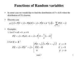
2. Functions of a Random Variable • the distribution of some function of X • supposeX is the rate atwhich customers are served in a queue • then 1/X is the average waiting time • If wehave the distribution of X, we should be able to: • determine the distribution of 1/X • or of any other function of X

3. Random Variable with a Discrete Distribution • Distance from the Middleexample • Let X have the uniform distribution on the integers1, 2, . . . , 9. • Suppose that we are interested in how far X is from the middle of thedistribution, namely, 5. • We could define Y = |X − 5| and compute probabilities suchas • Pr(Y = 1) = Pr(X ∈ {4, 6}) = 2/9.

4. Function of a Discrete Random Variable • Let X have a discrete distribution with p.f. f , • let Y = r(X) for some function of r defined on the set of possible values of X • For each possible value y of Y , the p.f. g of Y is

5. Distance from the Middle • The possible values of Y in thepreviousexample are 0, 1, 2, 3,and 4. • We see that Y = 0 if and only if X = 5 • g(0) = f (5) = 1/9. • For all othervalues of Y , there are two values of X that give that value of Y . For example, • {Y = 4} = {X = 1} ∪ {X = 9}. • So, g(y) = 2/9 for y = 1, 2, 3, 4.

6. Random Variable with a Continuous Distribution • If a random variableX has a continuous distribution, then the procedure for derivingthe probability distribution of a function of X differs from that given for a discretedistribution. • One way to proceed is by direct calculation

7. Average Waiting Time • Let Z be the rate at which customers are served in a queue, • suppose that Z has a continuous c.d.f. F. • The average waiting time is Y = 1/Z. • If we want to find the c.d.f. G of Y , we can write

8. Random Variable with a Continuous Distribution • In general, suppose that the p.d.f. of X is f and that another random variable isdefined as Y = r(X). • For each real number y, the c.d.f. G(y) of Y can be derived asfollows: • If the random variable Y also has a continuous distribution, its p.d.f. g can be obtainedfrom the relation

9. Direct Derivation of the p.d.f. • Let r be a differentiable one-to-one function on the open interval (a, b). • Then r is either strictly increasing or strictly decreasing. • Because r is also continuous,it will map the interval (a, b) to another open interval (α, β), called the image of(a, b) under r. • That is, for each x ∈ (a, b), r(x) ∈ (α, β), and for each y ∈ (α, β) there isx ∈ (a, b) such that y = r(x) and this y is unique because r is one-to-one. • So the inverses of r will exist on the interval (α, β), meaning that for x ∈ (a, b) and y ∈ (α, β) wehave r(x) = y if and only if s(y) = x.

10. Theorem • Let X be a random variable for which the p.d.f. is f and for which Pr(a <X<b) = 1. • Here, a and/or b can be either finite or infinite. • Let Y = r(X), and suppose that r(x)is differentiable and one-to-one fora <x <b. • Let (α, β) be the image of the interval(a, b) under the function r. • Let s(y) be the inverse function of r(x) for α <y <β. • Then the p.d.f. g of Y is

11. Proof • If r is increasing, then s is increasing, and for each y ∈ (α, β) • Because s is increasing, ds(y)/dy is positive; hence, it equals |ds(y)/dy| and thisequation impliesthetheorem. • Similarly, if r is decreasing, then s is decreasing, and foreach y ∈ (α, β), • Since s is strictly decreasing, ds(y)/dy is negative so that −ds(y)/dy equals |ds(y)/dy|. It follows that theequationimplies thetheorem.

12. TheProbabilityIntegralTransformation • Let X be a continuous random variable • Thep.d.f. f (x) = exp(−x) for x >0 and 0otherwise. • The c.d.f. of X is F(x) = 1− exp(−x) for x >0 and 0 otherwise. • If we letF be the function r, we can find the distributionof Y = F(X). • The c.d.f. or Y is, for 0 < y <1, • which is the c.d.f. of the uniform distribution on the interval [0, 1]. It follows that Yhas the uniform distribution on the interval [0, 1].

13. Theorem • LetX have a continuous c.d.f. F, • let Y = F(X). • This transformation from X to Y is called the probability integral transformation. • The distribution of Y is the uniform distribution on the interval [0, 1].

14. Proof • First, because F is the c.d.f. of a random variable, then 0 ≤ F(x) ≤ 1 for−∞ < x <∞. • Therefore, Pr(Y < 0) = Pr(Y > 1) = 0. • Since F is continuous, the setof x such that F(x) = y is a nonempty closed and bounded interval [x0, x1] for each yin the interval (0, 1). • Let F−1(y) denote the lower endpoint x0 of this interval, whichwas called the y quantile of F. • In this way, Y ≤ y if and only ifX ≤ x1. • Let G denote the c.d.f. of Y . Then • Hence, G(y) = y for 0 < y <1. Because this function is the c.d.f. of the uniformdistribution on the interval [0, 1], this uniform distribution is the distribution of Y .

15. Functions of Two or More Random Variables • When we observe data consisting of the values of several random variables, weneed to summarize the observed values in order to be able to focus on the informationin the data. • Summarizing consists of constructing one or a few functionsof the random variables. • We nowdescribe the techniques needed to determine the distribution of a function oftwo or more random variables.

16. Random Variables with a Discrete Joint Distribution • Suppose that n random variables X1, . . . , Xnhave a discrete joint distribution for which the joint p.f. is f, and that m functionsY1, . . . , Ym of these n random variables are defined as follows: Y1 = r1(X1, . . . , Xn), Y2 = r2(X1, . . . , Xn), ... Ym= rm(X1, . . . , Xn).

17. Random Variables with a Discrete Joint Distribution • For given values y1, . . . , ym of the m random variables Y1, . . . , Ym, let A denote theset of all points (x1, . . . , xn) such that r1(x1, . . . , xn) = y1, r2(x1, . . . , xn) = y2, ... rm(x1, . . . , xn) = ym. • Then the value of the joint p.f. g of Y1, . . . , Ym is specified at the point (y1, . . . , ym)by the relation

18. Random Variables with a ContinuousJoint Distribution • Suppose that the joint p.d.f. ofX = (X1, . . . , Xn)is f (x) and that Y = r(X). • Y = r(X1, . . . , Xn), • Thed.f. of Y can be calculated as follows: • If Y has a continuousdistribution, thenthederivation of G(y) givesthepd.f. of Y.

19. Direct Transformation of a Multivariate p.d.f. • Let X1, . . . , Xn have a continuous joint distributionfor which the joint p.d.f. is f . • Assume that there is a subset S of Rn such that • Pr[(X1, . . . , Xn) ∈ S]= 1. • Define n new random variables Y1, . . . , Yn as follows: Y1 = r1(X1, . . . , Xn), Y2 = r2(X1, . . . , Xn), ... Yn= rn(X1, . . . , Xn), wherewe assume that the n functions r1, . . . , rn define a one-to-one differentiabletransformation of S onto a subset T of Rn.

20. Direct Transformation of a Multivariate p.d.f. • Letthe inverse of this transformation begiven as follows: x1 = s1(y1, . . . , yn), x2 = s2(y1, . . . , yn), ... xn= sn(y1, . . . , yn).

21. Direct Transformation of a Multivariate p.d.f. • Then the joint p.d.f. g of Y1, . . . , Ynis • where J is the determinantand |J | denotes the absolute value of the determinant J . • This determinant J is called theJacobianof the transformation specified by the equations.

22. LinearTransformations • LetX = (X1, . . . , Xn) have a continuous joint distribution forwhich the joint p.d.f. is f . • Define Y = (Y1, . . . , Yn) by Y = AX, • whereA is a nonsingular n × n matrix. Then Y has a continuousjointdistributionwithp.d.f. • where A−1 is the inverse of A.