Download
1 / 20
270 likes | 786 Views
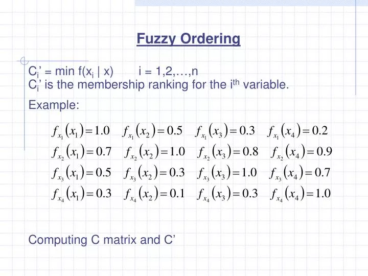
Fuzzy Ordering. C i ’ = min f(x i | x) i = 1,2,…,n C i ’ is the membership ranking for the i th variable. Example:. Computing C matrix and C’. Fuzzy Ordering. C =. The order is x 1 , x 4 , x 3 , x 2. Preference and Consensus. Crisp set approach is too restrictive.

E N D
Fuzzy Ordering Ci’ = min f(xi | x) i = 1,2,…,n Ci’ is the membership ranking for the ith variable. Example: Computing C matrix and C’
Fuzzy Ordering C = The order is x1, x4, x3, x2
Preference and Consensus Crisp set approach is too restrictive. Define reciprocal relation R iii = 0 rij + rji = 1 rij = 1 implies that alternative I is definitely preferred to alternative j If rij = rji = 0.5, there is equal preference. Two common measures of preference: Average fuzziness: Average certainty:
Preference and Consensus C is minimum, F maximum; rij = rji = 0.5 C is maximum, F minimum; rij = 1 0 1/2 1/2 1 They are useful to determine consensus. There are different types of consensus.
Antithesis of consensus M1: Complete ambivalence or maximally fuzzy M1 = M2: every pair of alternatives in definitely ranked All non-diagonal elements is 0 or 1. Alternative 1 is over alternative 2 M2 =
Antithesis of consensus Three types of consensus: Type 1: one clear choice and remaining (n-1) alternatives have equal secondary preference. (rkj = 0.5 k j) M1* = Alternative 2 has clear consensus.
Antithesis of consensus Type 2: one clear choice and remaining (n-1) alternatives have definite secondary preference. (rkj = 1 k j) M2* =
Antithesis of consensus Type 3: Fuzzy consensus Mf*: a unanimous decision and remaining (n-1) alternatives have infinitely many fuzzy secondary preference. Mf* = Cardinality of a relation is the number of possible combinations of that type.
(Type 1) (Type 1) (Type fuzzy) Antithesis of consensus
For M1 preference relation For M2 preference relation For M1* consensus relation For M2* consensus relation Distance to consensus
Example It does not have consensus properties. We compute: Notice m(M1) = 1 m(M2*) = 0 Complete ambivalence
Multi-objective Decision Making A = {a1,a2,…,an}: set of alternatives O = {o1,o2,…,or}: set of objectives The degree of membership of alternative a in Oj is given below. Decision function: The optimum decision a*
Multi-objective Decision Making Define a set of preferences {P} Parameter bi is contained on set {P}
Multi-objective Decision Making If two alternatives x and y are tied, Since, D(a) = mini[Ci(a)], there exists some alternative k, s.t. Ck(x) = D(x) and alternative g, s.t. Cg(y) = D(y) If a tie still presents, continue the process similar to the one above.
Fuzzy Bayesian Decision Method • First consider probabilistic decision analysis • S = {S1,S2,…,Sn} Set of states • P = {P(s1), P(s2),…, P(sn)} • P(si) = 1 P(si): probability of state I. It is called “prior probability”, expressing prior knowledge A = {a1, a2,…, am}, set of alternatives. For aj, we assign a utility value uji if the future state is Si
Fuzzy Bayesian Decision Method Utility matrix Associated with the jth alternative
Fuzzy Bayesian Decision Method Example: Decide if should drill for natural gas. a1: drill for gas a2: do not drill u11: the decision is correct and big reward +5 u12: decision wrong, costs a lot –10 u21: lost –2 u22: 4 U = 5 -10 -2 4
Decision Tree utility a1 S1 0.5 u11 = 5 S2 0.5 u12 = -10 a2 S1 0.5 u11 = -2 S2 0.5 u12 = 4 E(u1) = 0.5 5 + 0.5 (-10) = 2.5 E(u2) = 0.5 (-2) + 0.5 (4) = 1 So, E(u2) is bigger, this is from the alternative a2, the decision “ not drill” should be made. Should you need more information? Fuzzy Bayesian Decision Method
Fuzzy Bayesian Decision Method X = {x1,x2,…,xr} from r experiments or observations, used to update the prior probabilities. 1. New information is expressed in conditional probabilities.
The value of information V(x): X = {x1,x2,…,xr} imperfect information V(x) = E(ux*) – E(u*) Perfect information is represented by posterior probabilities of 0 or 1. Perfect information Xp The value of perfect information Fuzzy Bayesian Decision Method