Download
1 / 30
340 likes | 587 Views
Mapping GIS data. Entering and Storing data on GIS is OK, but not much fun. We want to look at the maps and see them at a bunch of different scales! sounds pretty easy, but be aware When you print a map, the scale is fixed to the paper;

E N D
Mapping GIS data Entering and Storing data on GIS is OK, but not much fun. We want to look at the maps and see them at a bunch of different scales! sounds pretty easy, but be aware When you print a map, the scale is fixed to the paper; When you view it on screen, It changes depending on the level of magnification In short, what looks good on screen may not look good on paper and vice versa
Map scales • Typically shown on paper maps a number of ways • Fractional scale--> 1:24,000; 1:62,500, etc. • Ratio of Map world to Real world in the same units • Bar scale--> a ruler that converts the map distance to the real world distance 1 mi 0 mi 0.125 0.25 0.375 0.5 0.66
Scales • Large scale maps show Small areas and • Small scale maps show Large areas • Because they’re fractional representations of the real world 1/24000 is a larger fraction than 1/62500 Thus the 1/24000 map shows a smaller area at higher level of detail or resolution
Map data • Technically, stored data have no scale • They have x, y -coordinates • They will get a scale when you view them or print them • Practically, data are collected at some scale that best suits them. • e.g.- a small scale map of the US that is scanned or digitized is not useful for making maps of larger scale data such as county roads
Scale issues of original data State boundary drawn to cover entire state was collected at much smaller scale than voting district lines, each of which is at a very large scale
Issues with data • Collect too much data and bogs down the machine trying to display the data • Too little data and there isn’t enough accuracy • that may significantly affect any interpretations of the data
Map Types • Different demands require different types of maps • Dependent on the data being used. • Different maps can have many symbols, or only one symbol. • Depends on what you’re trying to show. • Maps might use • Nominal data- names or ID’s objects • Categorical data- separates data into groups or classes • Ordinal data- separates data based on quantitative rank • Numerical data- data based on numbers with a standard interval between them
A single symbol map each pink shaded polygon is a state
Categorical Data points lines polygons
Nominal data • Data identified or named by some type of label • Can be text or number • Maps often have many objects, almost all of which have points, lines and polygons that are identified as some unique feature • Points may be a city or house • Lines may be rivers, faults, railroads, roads, etc. • Polygons may be parks, states, counties, countries, etc.
Ordinal data • Data are grouped by rank according to some quantitative measure • Cities may be small medium or large • Students may earn A B C or D’s in class • Soils may have I, II, III, IV infiltration • The data must be represented by unique values maps and colors must show or portray an increasing sense of value
A geological map is a Unique Values Map based on categorical data representing different formations, or other geological units
Numerical data • Numbers that represent continuous phenomena that fall along a regularly spaced interval • Rainfall, elevations, populations, chemical concentrations, etc. • Equal changes in the interval involve equal changes in the thing being measured • Ratio vs Interval numerical data • Ratio measured with respect to some meaningful zero point • Ex.- Rainfall; if zero, then no rain has fallen • Can add, subtract, multiply and divide these data • Interval measured against no meaningful zero point • Ex.- Temperature in F or C scale; has a regular scale, but zero on the thermometer does not mean a total lack of temperature. • Any data that can have a negative value is Interval (e.g. elevation) • Interval can only support addition and subtraction
Symbols associated with numerical data • Points and Lines typically arranged so that the bigger the numerical attribute number, the larger the point or the thicker the line • Graduated Symbols- Points and lines are divided into classes with a given range of values for each class and a symbol unique to that class • A classed map • Proportional Symbols- numeric value is proportional to the size of the symbol • Creates what is referred to as an unclassed map
Classed map Unclassed map
Symbols associated with numerical data • Polygons-numeric data are typically represented by colors • Can vary by hue, saturation or intensity • Changes in rainfall are commonly represented this way with each class a deeper shading of the color (intensity) for that shape
Graduated color maps or Choropleth maps Two varieties of precipitation maps using color intensity The top map uses a monochromatic intensity ramp to represent various increasing amounts of annual rainfall The bottom is a two toned color ramp of the same data, with yellow = dryer and green = wetter
Normalized data • Some features will have larger symbols due to larger attribute values associated with larger coverages or areas • Larger counties will often have more farmland or larger populations, but it will be spread out over larger areas. • Normalizing the population to area (people divided by square miles) keeps the symbols from being disproportionally larger and therefore seemingly more important
Dot density maps can normalize the data by letting each dot represent 1 million people. the more dots, the more people in that state. Can be arranged in specific locations in the state too
Classifying (grouping) data • Many methods for grouping numeric data • Depends what you want to show • Natural breaks (Jenks)- looks for gaps in data values • Equal interval-equal size for the intervals • Defined interval- range of values defined by user • Quantile- same number of features in each class • Class defined • Geometric interval- each class multiplied by a coefficient to create the next class • Standard deviation- the statistical deviation from normal of the data in any attribute field • Manual (arbitrary) breaks- self explanatory
Raster data • Two types of rasters • Thematic Raster and Image raster • Thematic- 2 categories • Discrete- coded values identify discrete regions of similar values • e.g., geology or land use • Continuous- values change continuously from one location to another • e.g., elevation or precipitation • Image- from satellites and photos • Pixels are given lightness/darkness values from 0-255 with 0 being black and 255 being white
Discrete raster • Best using Unique Values classification • Each value receives a color • Geology map example on next slide Continuous raster • Classified • Values divided into classes and classes are given colors • Elevation map example on next slide • Stretched • Values are scaled to one of 256 color shades • Elevation map c) on next slide
a) Thematic raster discrete unique values- geology b) Thematic raster continuous classified values- elevation
Image raster • Stretched vs Composite • Stretched - applied to single bandwidth images • i.e., grayscale images • Uses same as the stretched process does in the thematic raster continuous data values • Assumes normally distributed pixel data • Composite uses RGB color bandwidths • Varies values from 0 to 255 per bandwidth • 255 R with low G and B -makes red • 255 R and G with low B - makes yellow • Each bandwidth may be stretched as well
Stretching the values on a single band image - a one std dev stretch
RGB composite Stretched green bandwidth