Download
1 / 45
450 likes | 490 Views
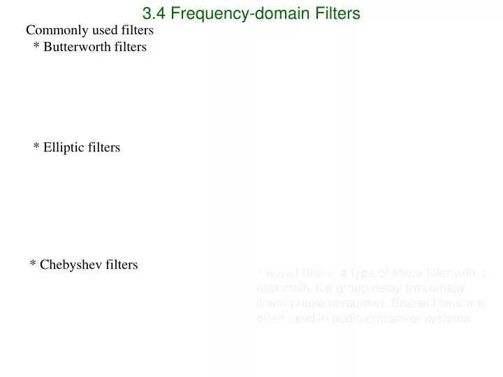
3.4 Frequency-domain Filters. Commonly used filters * Butterworth filters * Elliptic filters * Chebyshev filters. * Bessel filters a type of linear filter with a maximally flat group delay (maximally linear phase response). Bessel filters are often used in audio crossover systems.

E N D
3.4 Frequency-domain Filters Commonly used filters * Butterworth filters * Elliptic filters * Chebyshev filters * Bessel filters a type of linear filter with a maximally flat group delay (maximally linear phase response). Bessel filters are often used in audio crossover systems.
Maturity in analog lowpass filter design (1. (2. (3.
3.4.1 Removal of high-frequency noise: Butterworth lowpass filters Properties of Butterworth filters: 1. Most commonly used frequency-domain filters 2. Simplicity 3. A maximally flat magnitude response in the pass-band 4. 2N 1 derivatives of the squared magnitude response at ( = 0) = 0, for Butterworth lowpass filter of order N 5. Monotonic filter response in the pass-band and the stop-band 6. The squared transfer function |Ha(j)|2 =1/[1+( j/jc)2N] Ha: the frequency response of the analog filter c: the cutoff frequency (in radians/s) 7. Completely specified by the cutoff frequency c and the order N. 8. N increases more flat pass-band response; sharper pass-band to stop-band transition
Properties of Butterworth filters: 9. |Ha(jc)|2 = 1/2 for all N 10. The squared transfer function Ha(s) Ha(s) =1/[1+( s/jc)2N] 11. The poles of the squared transfer function sk = c exp{j[1/2 + (2k 1) / 2N]}, k = 1, 2, 3, …, 2N (a) For the filter coefficients to be real complex poles must appear in conjugate pairs (b) For a stable and causal responser Ha(s) only has poles on the left-hand side of the s-plane Ha(s) = G/[(sp1) (sp2) (sp3)…(spN)] 12. By using the bilinear transform s = (2/T)[(1 z1)/(1 + z1)] to map Ha(s) to the z-domain, H(z) = G’(1 + z 1)N/(Nk = 0 ak zk), k = 0, 1, 2, …, N a0 = 1 G’ is such that H(z) = 1 at z = 1, i.e., at DC y(n) = Nk = 0 bk x(n-k) - Nk = 0 ak y(n-k) 13. H(z) is an IIR filter
Step 1 1.
Step 2: Pole locations S(1) = -0.5561 + 1.3425i S(2) = -1.3425 + 0.5561i S(3) = -1.3425 - 0.5561i S(4) = -0.5561 - 1.3425i S(5) = 0.5561 - 1.3425i S(6) = 1.3425 - 0.5561i S(7) = 1.3425 + 0.5561i S(8) = 0.5561 + 1.3425i
Step 3: Form Ha(s) Choose s(1:4) as the poles for Ha(s) Ha(s) = 分子 /(s – s(1)) (s – s(2)) (s – s(3)) (s – s(4)) Ha(s) = 1 @ DC , so the 分子 = 2.111456 * 2.111456 = 4.458247 Ha(s) = 4.458247 /(s – s(1)) (s – s(2)) (s – s(3)) (s – s(4)) (equation 3.62)
S = (2/T)(1-z-1)/(1+z-1) • Ha(s) = 4.458247 /(s – s(1)) (s – s(2)) (s – s(3)) (s – s(4)) • H(z) = Equation 3.63 • b = [0.0465829, …. • a = [1, -0.776740, ….. • Use [h,w] = freqz(b,a) • fs = 200; • a = [1, -0.776740, 0.672706, -0.180517,0.029763]; • b = [0.0465829, 0.186332,0.279497,0.186332,0.046583]; • % a = [1.0000 -0.7767 0.6727 -0.1805 0.0298]; • % b= [0.0466 0.1863 0.2795 0.1863 0.0466]; • [h,w] = freqz(b,a); • subplot(2,1,1); • plot(w*(fs/2)/pi,abs(h));xlabel('Frequency, Hz'); ylabel('Magnitude'); grid; • subplot(2,1,2); • plot(w*(fs/2)/pi,angle(h) * 180 / pi); xlabel('Frequency, Hz'); ylabel('Phase, degree'); grid; • fvtool(b,a); Sep 4: Bilinear transform
[b,a] = butter(4,0.4); fvtool(b,a); % The four zeros are at the same location.
a = [1, -0.776740, 0.672706, -0.180517,0.029763]; b = [0.0465829, 0.186332,0.279497,0.186332,0.046583]; fvtool(b,a);
a = [1.0000 -0.7767 0.6727 -0.1805 0.0298]; b= [0.0466 0.1863 0.2795 0.1863 0.0466]; fvtool(b,a);
Step 5 y(n) = Nk = 0 bk x(n-k) - Nk = 0 ak y(n-k) (Equation 3.59)
Homeworkdue on 2009.11.16 (Monday midnight) Design a Butterworth LPF with N = 4, fc = 50 Hz. (fs = 200 Hz) (i) Ha(s) = ? (ii) H(z) = ? (iii) Plot the magnitude response and the phase response. Put the answers in a Word file and turn in on the Black Board System before the midnight of 2009.11.16.
Design by Matlab B = [0.0466 0.1863 0.2795 0.1863 0.0466] A = [1.0000 -0.7821 0.6800 -0.1827 0.0301] H(z) = (0.0466 + 0.1863 z-1 + 0.2795 z-2 + 0.1863 z-3 + 0.0466 z-4) / (1.0000 - 0.7821 z-1 + 0.6800 z-2 - 0.1827 z-3 0.0301 z-4)
To compensate for the distortion caused by bilinear transform
Figure 3.06(Original ECG signal with baseline wandering Figure 3.27(Output of derivative-based time-domian highpass filter as shown in Figure 3.27 Figure 3.38(Output of Butterworth highpass filter
Figure 3.27 Figure 3.39