Download
1 / 27
270 likes | 406 Views
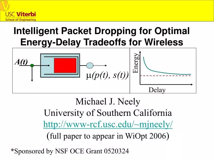
A(t). Energy. m (p(t), s(t)). Delay. Intelligent Packet Dropping for Optimal Energy-Delay Tradeoffs for Wireless. Michael J. Neely University of Southern California http://www-rcf.usc.edu/~mjneely/ ( full paper to appear in WiOpt 2006 ). *Sponsored by NSF OCE Grant 0520324. Good. A(t).

E N D
A(t) Energy m(p(t), s(t)) Delay Intelligent Packet Dropping for Optimal Energy-Delay Tradeoffs for Wireless Michael J. Neely University of Southern California http://www-rcf.usc.edu/~mjneely/ (full paper to appear in WiOpt 2006) *Sponsored by NSF OCE Grant 0520324
Good A(t) rate m Med m(P(t), S(t)) Bad power P Time slotted system (t {0, 1 , 2, …}) t 0 1 2 3 … Assumptions: Random Arrivals A(t) i.i.d. over slots. (Rate l bits/slot) 2) Random Channel states S(t) i.i.d. over slots. 3) Transmission Rate Function P(t) --- Power allocation during slot t S(t) --- Channel state during slot t m(P(t), S(t))
A(t) m(P(t), S(t)) Fundamental Energy-Delay Tradeoff Theory and the Berry-Gallager Bound: Avg. Power Avg. Delay F(l) = Min. Avg. Energy Required for Stability [Berry 2000, 2002]
Fundamental Energy-Delay Tradeoff Theory and the Berry-Gallager Bound: Avg. Power O(1/V) Avg. Delay V V In terms of a dimensionless index parameter V>0: [Berry 2000, 2002]
Fundamental Energy-Delay Tradeoff Theory and the Berry-Gallager Bound: O(1/V) Avg. Power Avg. Delay V V In terms of a dimensionless index parameter V>0: [Berry 2000, 2002]
Fundamental Energy-Delay Tradeoff Theory and the Berry-Gallager Bound: O(1/V) Avg. Power Avg. Delay V V In terms of a dimensionless index parameter V>0: [Berry 2000, 2002]
Fundamental Energy-Delay Tradeoff Theory and the Berry-Gallager Bound: O(1/V) Avg. Power Avg. Delay V V In terms of a dimensionless index parameter V>0: [Berry 2000, 2002]
Fundamental Energy-Delay Tradeoff Theory and the Berry-Gallager Bound: Avg. Power O(1/V) Avg. Delay V V In terms of a dimensionless index parameter V>0: [Berry 2000, 2002]
Avg. Delay Fundamental Energy-Delay Tradeoff Theory and the Berry-Gallager Bound: Avg. Power O(1/V) V V Berry-Gallager Bound Assumes: Admissibility criteria Concave rate-power function i.i.d. arrivals A(t) 4. No Packet Dropping
r A(t) (rate l) (1-r) Our Formulation: Intelligent Packet Dropping m(P(t), S(t)) Control Variables: Goal: Obtain an optimal energy-delay tradeoff Subject to: Admitted rate >= rl ( 0 < r < 1 )
Energy-Delay Tradeoffs with Packet Dropping… O(1/V) Avg. Delay Avg. Power ? V V F* = F(lr) = New Min. Average Power Expenditure (required to support rate rl). r A(t) (rate l) (1-r)
Energy-Delay Tradeoffs with Packet Dropping… O(1/V) Avg. Delay Avg. Power ? V V F* = F(lr) = New Min. Average Power Expenditure (required to support rate rl). r A(t) (rate l) (1-r)
Energy-Delay Tradeoffs with Packet Dropping… ? O(1/V) Avg. Delay Avg. Power V V F* = F(lr) = New Min. Average Power Expenditure (required to support rate rl). r A(t) (rate l) (1-r)
Energy-Delay Tradeoffs with Packet Dropping… ? O(1/V) Avg. Delay Avg. Power V V F* = F(lr) = New Min. Average Power Expenditure (required to support rate rl). r A(t) (rate l) (1-r)
An Example of Naïve Packet Dropping: Random Bernoulli Acceptance with probability r. O(1/V) Avg. Delay Avg. Power F* = F(lr) V V Consider a system that satisfies all criteria for the Berry-Gallager bound, including i.i.d. arrivals every slot. After random packet dropping, arrivals are still i.i.d…. r A(t) (rate l) (1-r)
An Example of Naïve Packet Dropping: Random Bernoulli Acceptance with probability r. O(1/V) Avg. Delay Avg. Power F* = F(lr) V V Consider a system that satisfies all criteria for the Berry-Gallager bound, including i.i.d. arrivals every slot. After random packet dropping, arrivals are still i.i.d., and hence performance is still governed by Berry-Gallager square root law. r A(t) (rate l) (1-r)
But here we consider Intelligent Packet Dropping: achievable! O(1/V) Avg. Delay Avg. Power F* = F(lr) V V Thus: The square root curvature of the Berry Gallager bound is due only to a very small fraction of packets that arrive at innopportune times. r A(t) (rate l) (1-r)
Algorithm Development: A preliminary Lemma: Lemma: If channel states are i.i.d. over slots: For any stabilizable input rate l, there exists a stationary randomized algorithm that chooses power P*(t) based only on the current channel state S(t), and yields: *This is an existential result: Constructing the policy could be difficult and would require full knowledge of channel probabilities.
Algorithm 1: (Known channel probabilities) The Positive Drift Algorithm: Step 1 -- Emulate a finite buffer queueing system: A(t) U(t) Q = max buffer size
Step 2 -- Apply the stationary policy P*(t) such that: (where r < r + e < 1) rate (r+e)l rate l Positive drift! mmax 0 Q
Step 2 -- Apply the stationary policy P*(t) such that: (where r < r + e < 1) rate (r+e)l rate l Positive drift! mmax 0 Q Choose: e = O(1/V) , Q = O(log(V))
Algorithm 2: (Unknown channel probabilities) Constructing a practical Dynamic Packet Dropping Algorithm: m(P(t), S(t)) rate l U(t) …but we still want to maintain mav at least (r+e)l… mmax 0 Q Define the Lyapunov Function: L(U) L(U) = ew(Q-U) U 0 Q
(r + e)lmav < A(t) (rate l) m(P(t), S(t)) U(t) Want to ensure: Use the “virtual queue” concept for time average inequality constraints [Neely Infocom 2005] m(P(t), S(t)) X(t) (r+e)A(t)
Let Z(t) := [U(t); X(t)] Form the mixed Lyapunov function: Define the Lyapunov Drift: Lyapunov Optimization Theory [Neely, Modiano 03, 05]: Similar to concept of “stochastic gradient” applied to a flow network -- [Lee, Mazumdar, Shroff 2005]
The Dynamic Packet Dropping Algorithm: Every timeslot, observe: Queue values U(t),X(t) and Channel State S(t) 1. Allocate power P(t) that solves: 2. Iterate the virtual queue X(t) update equation with 3. Emulate the Finite Buffer Queue U(t).
Theorem: For the Dynamic Packet Dropping Alg. achievable! O(1/V) Avg. Delay Avg. Power F* = F(lr) V V
Conclusions: The Dynamic Algorithm does not require knowledge of channel probabilities, and yields a logarithmic power-delay tradeoff. Intelligent Packet Dropping Fundamentally improves the Power-delay tradeoff (from square root law to logarithm). Further: For a large class of systems, the [O(1/V), O(log(V))] tradeoff is necessary! Energy-Delay Tradeoffs for Multi-User Systems [Neely Infocom 06] “Super-fast” flow control for utility-delay tradeoffs [Neely Infocom 06]