Functional linear models

1. Functional linear models

2. Three types of linear model to consider: • Response is a function; covariates are multivariate. • Response is scalar or multivariate; covariates are functional. • Both response and covariates are functional.

3. Functional response with multivariate covariates • Response: yi(t), i=1,…,N • Covariate: xi1,…, xip • Model:

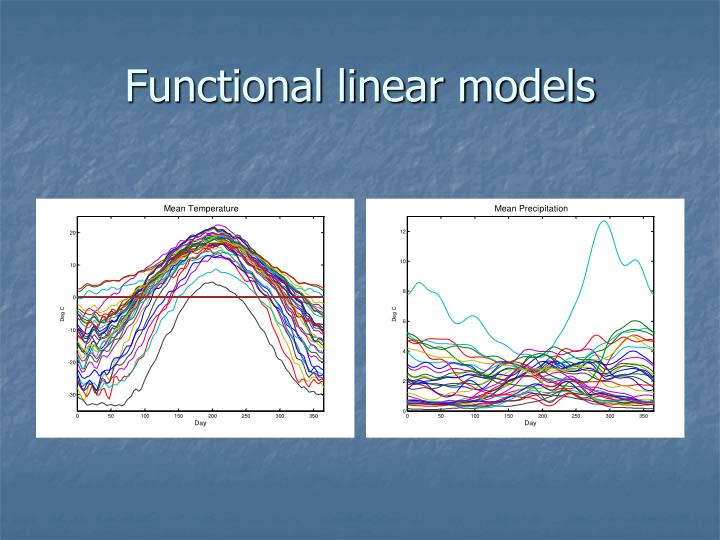
4. How does daily temperature depend on climate zone? • 35 Canadian temperature stations, divided into four zones: Atlantic, Pacific, Continental, and Arctic. • Response is 30-year average daily temperature. • A functional one-way analysis of variance, set up to have a main effect, and zone effects summing to zero.

5. Analyzing the data • This is straightforward. • If Y(t) is the N-vector of response functions, β(t) is the 5-vector of regression functions (main effect + zone effects), then the LS estimate is • β(t) = (X’X)-1X’ Y(t) .

6. Main and zone effect functions

7. Assessing effects • We probably want to assess effects pointwise: For what times t is an effect substantial? • This can be done using F-ratios conditional on t, pointwise confidence bands, etc. • The multiple comparison problem is especially challenging here.

8. Response is scalar, Covariate is a single functional variable • Response: yi , i=1,…,N • Covariate: xi (t) • Model:

9. We have to smooth! • The technical and conceptual issues become much more interesting when the covariate is functional. • A functional covariate is effectively an infinite-dimensional predictor for a finite set of N responses. We can fit the data exactly! • Smoothing becomes essential; without it, β(t) will be unacceptably rough, and we won’t learn anything useful.

10. Predicting log annual precipitation from the temperature profiles • Can we determine how much precipitation a weather station will receive from the shape of the temperature profile? • What roughness penalty should we use to smooth β(t) ? • We penalize the size of (2π/365)2Dβ+D3β, the harmonic acceleration of β(t) . This smooths towards a shifted sinusoid.

11. The smoothed regression function • Annual precipitation is determined by: (1) spring temperature, and (2) by the contrast between late summer and fall temperatures.

12. The fit to the data • The fit is good. • We see clusters of hi-precip. marine stations, and of continential stations. • Arctic stations have the least precip.

13. What about both the response and covariate being functional? • Response y(t), covariate x(s) or x(s,t). Here we have a lot of possibilities. We can predict y(t) using the shape of x(s,t) over: • all of s, especially for periodic data, • only at s = t, concurrent influence only, or for some delay s = t – δ, • s  t, no feed forward, • some region Ωt depending on t.

14. Predicting the precipitation profile from the temperature profile • The model is: In this case we have to smooth β(s,t) with respect to both s and t.

15. The regression function

19. The concurrent model • This time, we’ll only use temperature at time t to predict precipitation at time t:

20. The regression functions The influence of temperature is nearly constant over the year. Let’s see how the two fits compare.

24. The historical linear model • When the functions are not periodic, it may not be reasonable to assume that x(s) can influence y(t) when s > t. • The historical linear model is described in Applied Functional Data Analysis, and in talk at this conference by Nicole Malfait.

25. The concurrent model and differential equations • One important extension of the concurrent model is to the fitting of data by a differential equation. • A simple example is