Download

1 / 39

E N D
Example. The R data frame milk, available from the course web page, records, for each of 9 regions of the USA, the average peak radioactivity (radiation x in picocuries/L) in milk samples following the Chernobyl accident in 1986 and the percentage increase in death rates (percent y) in the following summer.
radiation percent Middle.Atlantic 23 2.2 South.Atlantic 20 2.4 New.England 22 1.9 East.North-Central 29 3.9 West.North-Central 32 3.6 East.Southern 21 2.6 Central.Southern 16 0.0 Mountain 37 4.2 Pacific 44 5.0
The next graph shows a plot of percent y against radiation x, Two individual points have been labelled with the R function “identify”. > plot(percent~radiation) > identify(percent~radiation, labels=row.names(milk))
It seems reasonable to consider a linear model and the next graph shows the corresponding fitted relation. The model is fitted and the plot is drawn in R with > plot(percent~radiation) > milk.lm=lm(percent~radiation) > abline(milk.lm)
The object we have called milk.lm stores much information associated with the fit of the model. This can be extracted with various R functions, e.g. summary, coef, residuals. Here is some of the output from the function summary:
This leads to the regression equation percent = 0.14925 x radiation – 1.17961
Note that the estimate of the coefficient b associated with radiation is 0.14925 while its standard error is only 0.02543. The ratio of these is 5.87. Hence if we believe the model is reasonable, then in particular b is certainly nonzero, and so the distribution of the percentage increase in death rates does indeed depend on the radioactivity level as measured in milk samples.
However, it is not possible to say whether this observed statistical association is causal, or whether there is some third unobserved variable accounting in some sense for the variation in both the variables above.
The correlation coefficient, r, is calculated using the command > cor(percent,radiation) [1] 0.9116522 r is a number between -1 and +1 and the closer it is to 1 or -1 the better the “fit” of the straight line to the data. 0 represents a poor fit. 0.9116522 indicates a good linear relation here. N.B. Treat r values with caution (see later)
Residuals The residuals should be thought of as what is left of the values of the response variable after the fit has been subtracted. Ideally they should show no further dependence (especially no further location dependence) on x.
In general this should be investigated graphically by plotting residuals against the explanatory variable(s) x. For linear models, we frequently compromise by plotting residuals against fitted values.
For the “milk” data, the residuals are obtained with the following command
Note the slight pattern in the residuals: tending to be negative, then positive, then negative, as radiation increases, suggesting perhaps some nonlinearity in the dependence of percent on radiation. However, 9 observations are quite insufficient to settle this point.
It is important to remember in analysis of results that while summary statistics (like r) are helpful, they are not sufficient. Good diagnostics are typically based on case analysis, i.e. an examination of each observation in turn in relation to the fitting procedure. This is why residuals are so useful.
Example: Anscombe’s Artificial Data The R data frame anscombe is made available by > data(anscombe) This contains 4 artificial datasets, each of 11 observations of a continuous response variable y and a continuous explanatory variable x.
All the usual summary statistics related to the classical analyses of the fitted models are identical across the 4 datasets. This includes the coefficients a and b and the correlation coefficient, r.
Consideration of the residuals shows that very different judgements should be made about the appropriateness of the fitted model to each of the 4 cases. The ideal situation is for the residuals to show a random pattern with no further dependence on the explanatory variable.